Stage 1b: Time-Zone Traffic Profiles

1 Why time-zone profiles matter

Stage 1a estimates total daily traffic (AADT) for every road link. This is sufficient for computing collision rates — collisions per million vehicle-kilometres — but it treats all hours of the day as equivalent. In practice, risk varies significantly by time of day: peak-hour traffic is denser, faster, and involves more interactions than overnight flow.

Stage 1b estimates the shape of the daily traffic profile for every road link: what fraction of daily traffic flows in each time band? Combined with the Stage 1a AADT estimate, this gives per-hour flow rates for any road in the network.

2 Time bands

WebTRIS annual reports provide cumulative flow totals for four hour windows. Differencing these gives four non-overlapping time bands:

Code label	True period	Hours
core_daytime_frac	07:00–18:59	12
shoulder_frac	06–07 + 19–22 (mixed shoulder)	4
late_evening_frac	22:00–24:00	2
overnight_frac	00:00–06:00	6

The model predicts the fraction of daily traffic in each band. Absolute per-hour flow is then reconstructed as:

\[\text{flow\_ph\_peak} = \text{AADT} \times \frac{\text{peak\_frac}}{12}\]

3 Data and model setup

from pathlib import Path
import numpy as np
import pandas as pd
import matplotlib.pyplot as plt
from road_risk.config import _ROOT as ROOT

webtris = pd.read_parquet(ROOT / "data" / "processed" / "webtris" / "webtris_clean.parquet")

profiles_path = ROOT / "data" / "models" / "timezone_profiles.parquet"
profiles = pd.read_parquet(profiles_path) if profiles_path.exists() else pd.DataFrame()

road = pd.read_parquet(ROOT / "data" / "features" / "road_link_annual.parquet")
road_class_col = next(
    (c for c in ["road_classification", "road_type"] if c in road.columns), None
)

print(f"WebTRIS training sites : {webtris['site_id'].nunique():,} sites × "
      f"{webtris['year'].nunique()} years = {len(webtris):,} rows")
print(f"Profile estimates      : {len(profiles):,} rows" if not profiles.empty
      else "Profile estimates      : not found — run --stage profile")

WebTRIS training sites : 5,948 sites × 3 years = 15,011 rows
Profile estimates      : 21,675,570 rows

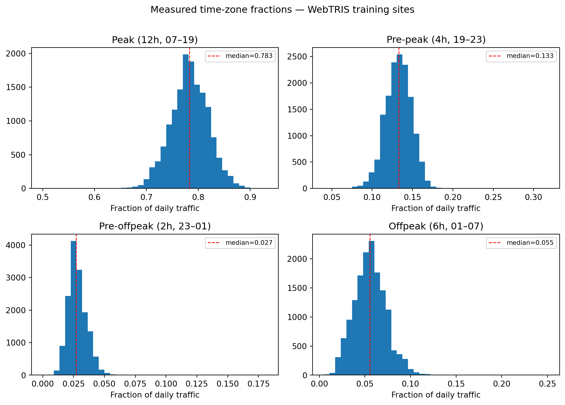
4 Training data: WebTRIS time-zone fractions

The profile model is trained on WebTRIS sensors — National Highways sites on motorways and major A-roads. For each site×year, the four time-band fractions are computed from the measured flow windows and used as prediction targets.

wt = webtris[webtris["all_flow"] > 0].copy()
wt["core_daytime_frac"]       = (wt["flow_ph_core_daytime"]       * 12) / wt["all_flow"]
wt["shoulder_frac"]    = (wt["flow_ph_shoulder"]     *  4) / wt["all_flow"]
wt["late_evening_frac"] = (wt["flow_ph_late_evening"]  *  2) / wt["all_flow"]
wt["overnight_frac"]    = (wt["flow_ph_overnight"]     *  6) / wt["all_flow"]

fracs = ["core_daytime_frac", "shoulder_frac", "late_evening_frac", "overnight_frac"]
print("Time-zone fraction distributions (measured WebTRIS sites):\n")
print(wt[fracs].describe(percentiles=[0.1, 0.25, 0.5, 0.75, 0.9]).round(3).to_string())

Time-zone fraction distributions (measured WebTRIS sites):

       core_daytime_frac  shoulder_frac  late_evening_frac  overnight_frac
count          15003.000      15003.000          15003.000       15003.000
mean               0.783          0.133              0.028           0.056
std                0.036          0.016              0.008           0.018
min                0.500          0.040              0.000           0.005
10%                0.737          0.112              0.019           0.033
25%                0.760          0.122              0.023           0.044
50%                0.783          0.133              0.027           0.055
75%                0.808          0.144              0.033           0.067
90%                0.829          0.153              0.038           0.077
max                0.933          0.318              0.182           0.251

fig, axes = plt.subplots(2, 2, figsize=(10, 7))
titles = ["Peak (12h, 07–19)", "Pre-peak (4h, 19–23)",
          "Pre-offpeak (2h, 23–01)", "Offpeak (6h, 01–07)"]
for ax, col, title in zip(axes.flat, fracs, titles):
    ax.hist(wt[col].dropna(), bins=40, edgecolor="none")
    ax.set_title(title)
    ax.set_xlabel("Fraction of daily traffic")
    ax.axvline(wt[col].median(), color="red", linestyle="--", linewidth=1,
               label=f"median={wt[col].median():.3f}")
    ax.legend(fontsize=8)
plt.suptitle("Measured time-zone fractions — WebTRIS training sites", y=1.01)
plt.tight_layout()
plt.show()

print("Peak–offpeak ratio (measured sites):")
print(wt["core_overnight_ratio"].describe(percentiles=[0.1,0.25,0.5,0.75,0.9]).round(2).to_string())

plt.figure(figsize=(7, 4))
plt.hist(wt["core_overnight_ratio"].clip(0, 30), bins=50, edgecolor="none")
plt.xlabel("Peak flow/hr ÷ offpeak flow/hr")
plt.ylabel("Count")
plt.title("Peak–offpeak ratio distribution (WebTRIS sites)")
plt.axvline(wt["core_overnight_ratio"].median(), color="red", linestyle="--", linewidth=1)
plt.tight_layout()
plt.show()

Peak–offpeak ratio (measured sites):
count    15003.00
mean         8.00
std          3.74
min          1.07
10%          4.81
25%          5.68
50%          7.07
75%          9.14
90%         12.44
max         91.56

5 Model performance

Five models are trained (one per target) using HistGradientBoostingRegressor with GroupKFold cross-validation grouped by site_id, preventing the same sensor from appearing in both train and validation folds.

Features: location (lat/lon), log(AADT), network betweenness, distance to major road, population density, year, COVID flag.

Note

Target	CV R²	Interpretation
core_daytime_frac	~0.65	Strong — peak shape driven by road function and location
shoulder_frac	~0.63	Strong — evening pattern correlates with urban density
overnight_frac	~0.53	Moderate — night freight patterns are more variable
late_evening_frac	~0.46	Weakest — short transition band with mixed signal
hgv_core_daytime_frac	~0.63	Strong — HGV peak timing is structurally driven

The MAE for all fraction targets is < 0.03, meaning the model predicts daily traffic fractions to within about ±3 percentage points on average.

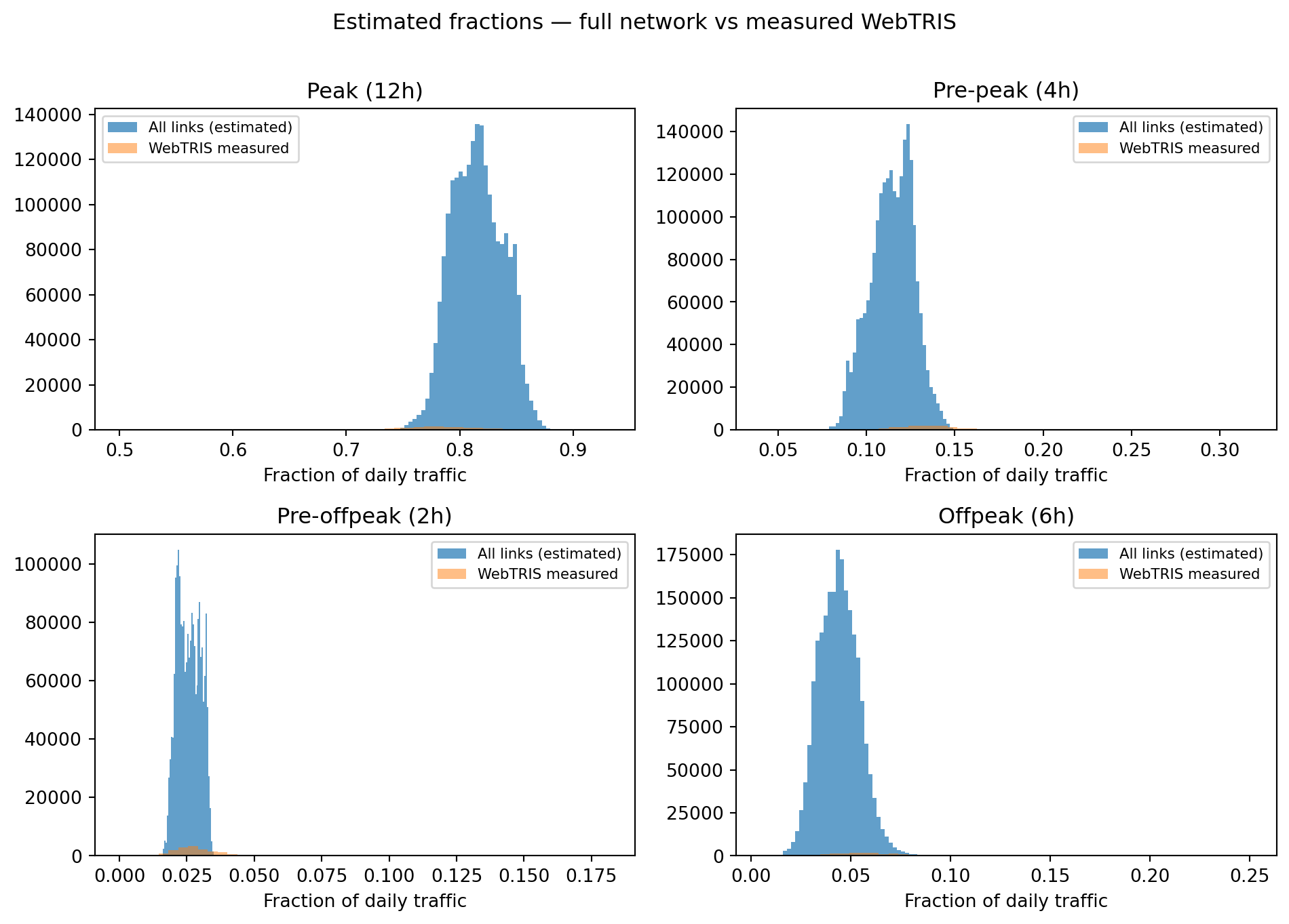
6 Estimated profiles across the full network

if not profiles.empty:
    latest = profiles[profiles["year"] == profiles["year"].max()].copy()
    print(f"Year {latest['year'].iloc[0]} — {len(latest):,} link estimates\n")
    frac_cols = [c for c in fracs if c in latest.columns]
    print(latest[frac_cols + ["core_overnight_ratio"]].describe(
        percentiles=[0.1, 0.25, 0.5, 0.75, 0.9]
    ).round(3).to_string())

Year 2024 — 2,167,557 link estimates

       core_daytime_frac  shoulder_frac  late_evening_frac  overnight_frac  core_overnight_ratio
count        2167557.000    2167557.000        2167557.000     2167557.000           2167557.000
mean               0.816          0.115              0.026           0.044                 9.824
std                0.023          0.012              0.004           0.010                 2.724
min                0.711          0.071              0.016           0.010                 3.274
10%                0.787          0.097              0.020           0.032                 6.971
25%                0.798          0.106              0.022           0.037                 7.879
50%                0.815          0.115              0.026           0.044                 9.249
75%                0.832          0.124              0.029           0.051                11.280
90%                0.847          0.129              0.032           0.057                13.322
max                0.894          0.166              0.041           0.112                44.646

if not profiles.empty:
    fig, axes = plt.subplots(2, 2, figsize=(10, 7))
    titles = ["Peak (12h)", "Pre-peak (4h)", "Pre-offpeak (2h)", "Offpeak (6h)"]
    for ax, col, title in zip(axes.flat, fracs, titles):
        if col in latest.columns:
            ax.hist(latest[col].dropna(), bins=50, edgecolor="none", alpha=0.7,
                    label="All links (estimated)")
            if col in wt.columns:
                ax.hist(wt[col].dropna(), bins=50, edgecolor="none", alpha=0.5,
                        label="WebTRIS measured")
            ax.set_title(title)
            ax.set_xlabel("Fraction of daily traffic")
            ax.legend(fontsize=8)
    plt.suptitle("Estimated fractions — full network vs measured WebTRIS", y=1.01)
    plt.tight_layout()
    plt.show()

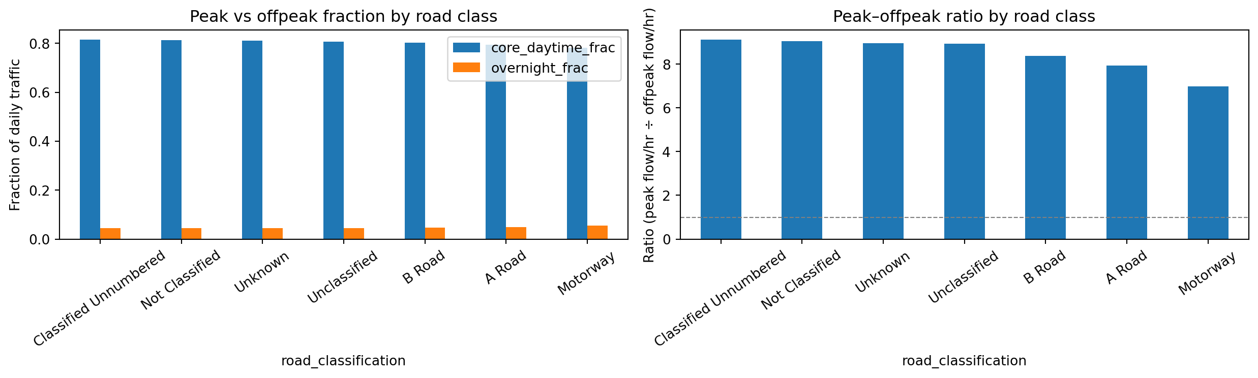
7 Profile variation by road class

Roads with different functions show distinct daily profiles. Motorways have high peak fractions (commuter + freight); rural unclassified roads have flatter profiles. The model captures this through road classification and network betweenness.

if not profiles.empty and road_class_col:
    with_class = profiles[profiles["year"] == profiles["year"].max()].merge(
        road[["link_id", road_class_col]].drop_duplicates("link_id"),
        on="link_id", how="left"
    )
    grp = (
        with_class.groupby(road_class_col)[["core_daytime_frac", "overnight_frac", "core_overnight_ratio"]]
        .median()
        .sort_values("core_daytime_frac", ascending=False)
    )
    print("Median time-zone fractions by road class:\n")
    print(grp.round(3).to_string())

    fig, axes = plt.subplots(1, 2, figsize=(13, 4))
    grp[["core_daytime_frac", "overnight_frac"]].plot(kind="bar", ax=axes[0])
    axes[0].set_title("Peak vs offpeak fraction by road class")
    axes[0].set_ylabel("Fraction of daily traffic")
    axes[0].tick_params(axis="x", rotation=35)

    grp["core_overnight_ratio"].plot(kind="bar", ax=axes[1])
    axes[1].set_title("Peak–offpeak ratio by road class")
    axes[1].set_ylabel("Ratio (peak flow/hr ÷ offpeak flow/hr)")
    axes[1].axhline(1, color="grey", linestyle="--", linewidth=0.8)
    axes[1].tick_params(axis="x", rotation=35)

    plt.tight_layout()
    plt.show()

Median time-zone fractions by road class:

                       core_daytime_frac  overnight_frac  core_overnight_ratio
road_classification                                                           
Classified Unnumbered              0.814           0.044                 9.112
Not Classified                     0.813           0.045                 9.045
Unknown                            0.810           0.045                 8.947
Unclassified                       0.806           0.045                 8.932
B Road                             0.802           0.048                 8.384
A Road                             0.793           0.050                 7.945
Motorway                           0.782           0.056                 6.975

8 Reconstructed per-hour flows

Using Stage 1a AADT estimates and Stage 1b fractions, per-hour flow rates can be computed for any link in the network.

if not profiles.empty:
    flow_cols = [c for c in [
        "flow_ph_core_daytime", "flow_ph_shoulder", "flow_ph_late_evening", "flow_ph_overnight"
    ] if c in profiles.columns]

    if flow_cols:
        sample_yr = profiles[profiles["year"] == profiles["year"].max()]
        print("Per-hour flow estimates — full network (vehicles/hour):\n")
        print(sample_yr[flow_cols].describe(
            percentiles=[0.25, 0.5, 0.75, 0.9, 0.99]
        ).round(1).to_string())

Per-hour flow estimates — full network (vehicles/hour):

       flow_ph_core_daytime  flow_ph_shoulder  flow_ph_late_evening  flow_ph_overnight
count             2167557.0         2167557.0             2167557.0          2167557.0
mean                  145.9              67.1                  29.6               16.8
std                   286.7             143.9                  63.4               38.2
min                     4.5               1.5                   0.6                0.3
25%                    31.6              13.0                   5.8                3.3
50%                    48.0              20.2                   9.3                5.2
75%                   113.0              50.1                  22.6               11.9
90%                   322.6             135.1                  59.5               32.5
99%                  1330.7             666.2                 291.6              177.4
max                  8756.3            4747.5                2398.6             1513.5

9 How this could feed into the collision model

The current production collision model uses total AADT as its exposure denominator. The per-hour flow rates from Stage 1b are produced for diagnostics and future temporal exposure weighting. A future Stage 2 model could use them to distinguish:

• Roads where most collisions occur during peak hours (high peak exposure)
• Roads with disproportionate night-time collisions (relative to low offpeak flow)

The core_overnight_ratio is also a candidate model feature, capturing whether a road functions primarily as a commuter route or serves mixed/freight traffic.

Note

Pipeline order

Stage 1a  python -m road_risk.model --stage traffic
            → data/models/aadt_estimates.parquet

Stage 1b  python -m road_risk.model --stage profile
            → data/models/timezone_profiles.parquet
            (requires Stage 1a)

Stage 2   python -m road_risk.model --stage collision
            → data/models/risk_scores.parquet

10 Known limitations

• WebTRIS training data is concentrated on motorways and major A-roads. Profiles for unclassified roads are extrapolated from location and network position rather than directly observed — the model assumes that road function and urban context are the dominant drivers of profile shape.
• The pre-offpeak band (23:00–01:00) has the weakest CV R² (~0.46) due to its short duration and mixed signal. Predictions for this band should be interpreted cautiously.
• Year-on-year variation in profiles (e.g. COVID impact on commuting patterns) is captured through the year_norm and is_covid features but may not fully reflect rapid behavioural shifts.