Open Road Risk
  • Home
  • Project
    • Project overview
    • Current model status
    • AI-assisted development
  • Background
    • Metrics and methodology
    • Literature evidence register
  • Literature
    • Crash frequency models
    • Exposure and traffic volume
    • Spatial methods and network risk
    • Junctions and conflict structure
    • Severity modelling
    • Validation and metrics
    • Transferability and open data limits
  • Data Sources
    • Overview
    • STATS19 Collisions
    • OS Open Roads
    • AADF Traffic Counts
    • WebTRIS Sensors
    • Network Model GDB
  • Methodology
    • Methodology Overview
    • Joining the Datasets
    • Feature Engineering
    • Empirical Bayes Shrinkage
  • Exploratory Data Analysis
    • Collision EDA
    • Collision-Exposure Behaviour
    • Vehicle Mix Analysis
    • Road Curvature
    • Months and Days of Week
    • Traffic Volume EDA
    • OSM Coverage
  • Models
    • Modelling Approach
    • Stage 1a: Traffic Volume
    • Stage 1b: Time-Zone Profiles
    • Stage 2: Collision Risk Model
    • Facility Family Split
    • Model Inventory
  • Outputs
    • Top-risk map
  • Future Work

On this page

  • 1 Why this matters
  • 2 What this page answers
  • 3 What STATS19 is
  • 4 How the data is collected
    • 4.1 Known reporting biases
  • 5 Use in practice
  • 6 Download
  • 7 Tables
  • 8 Key variables
    • 8.1 Collision table
    • 8.2 Vehicle table
    • 8.3 Casualty table
  • 9 Setup
  • 10 Load data
  • 11 Missingness and data quality
  • 12 Collision severity
    • 12.1 Overall distribution
    • 12.2 By road type
    • 12.3 By speed limit
  • 13 Temporal trends
    • 13.1 Year-on-year
    • 13.2 Monthly seasonality
    • 13.3 Day of week
    • 13.4 Hour of day
  • 14 Vehicle types
    • 14.1 Distribution
    • 14.2 HGV involvement by road type
    • 14.3 Vehicles per collision
  • 15 Geography
  • 16 Join quality
  • 17 Notes for clean.py
  • 18 Known issues

STATS19 — Road Casualty Statistics

1 Why this matters

Important

STATS19 is the outcome variable for this project. Every collision used to train and evaluate the risk model comes from this dataset. Its coverage, reporting biases, and severity classification directly shape what the model can and cannot learn.

Most road safety work in Great Britain is built on STATS19 because it is the only national, geocoded, severity-coded collision dataset. But it only records collisions that (a) involved personal injury and (b) were reported to the police. What it misses is as important as what it includes.

2 What this page answers

  1. What is STATS19 and what does it contain?
  2. How is the data collected, and what biases does that introduce?
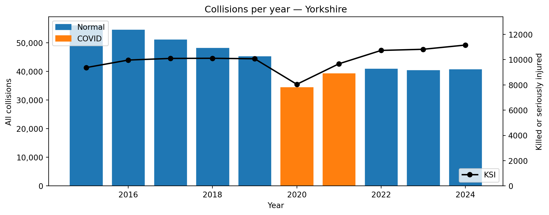
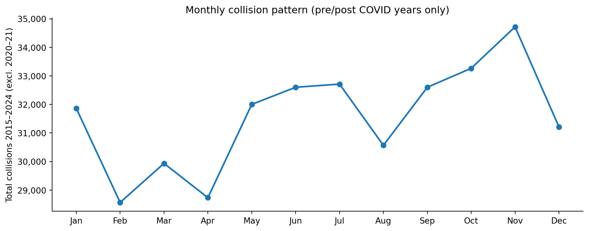
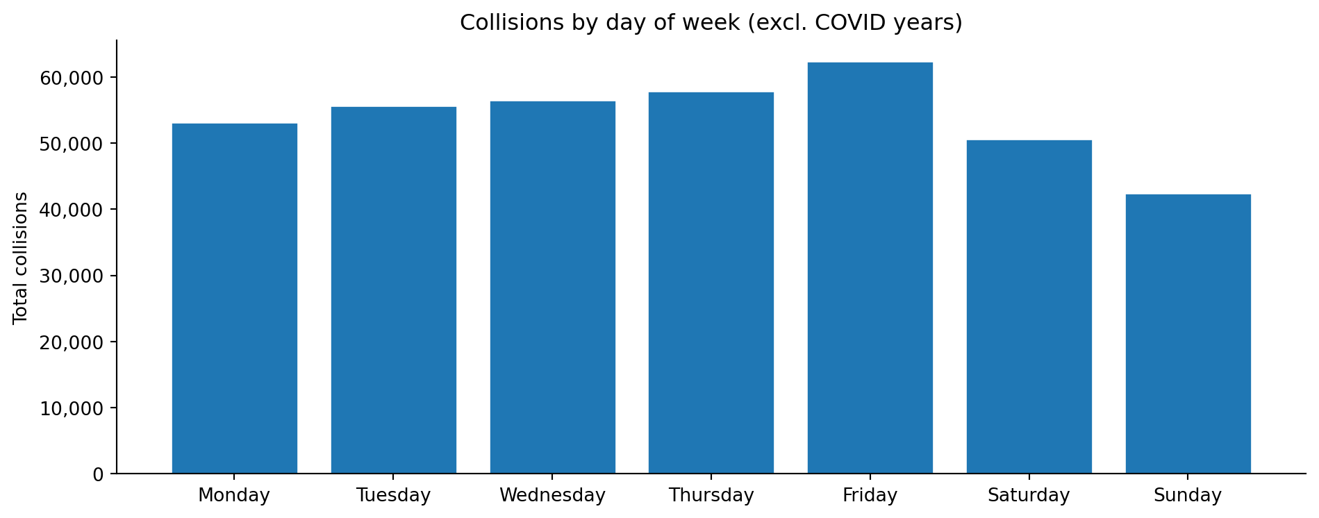
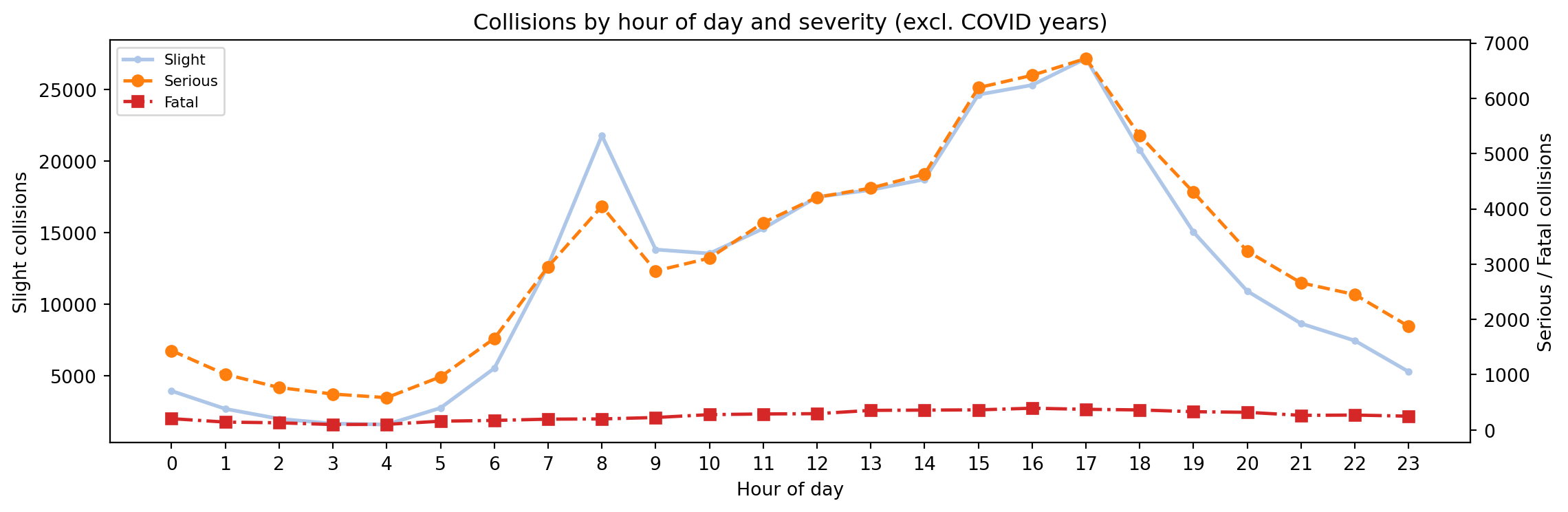
  3. What does the Northern and Central England sample look like over 2015–2024?
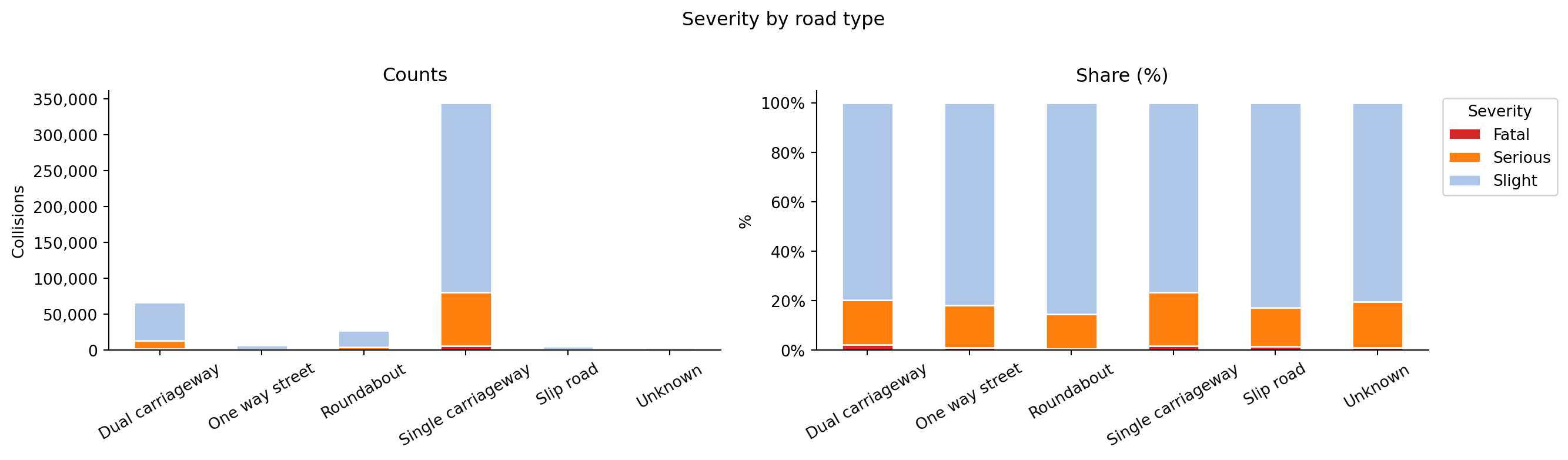
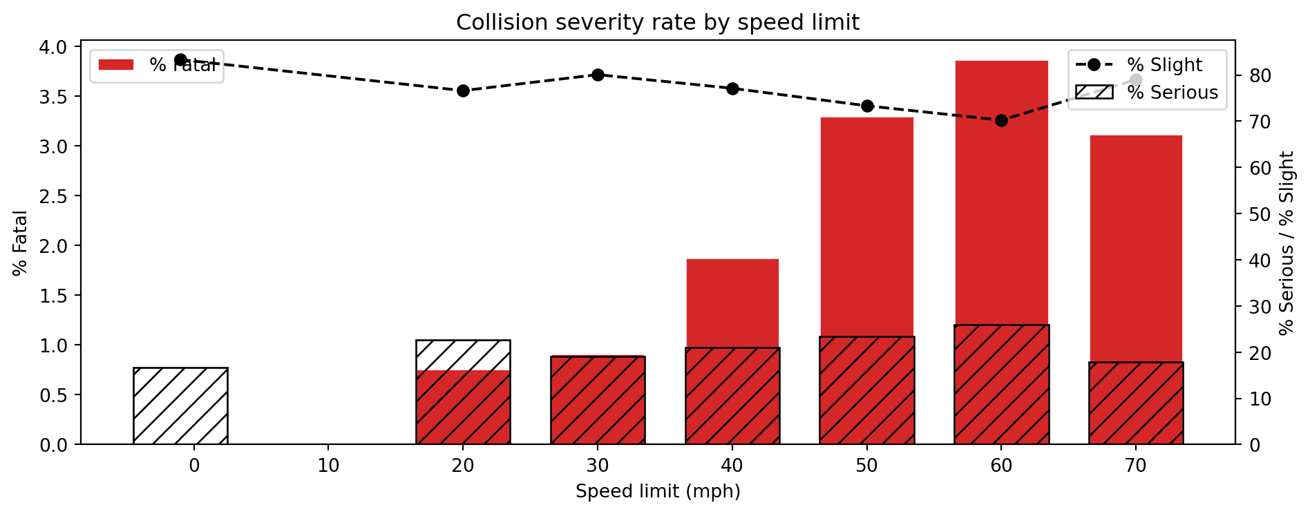
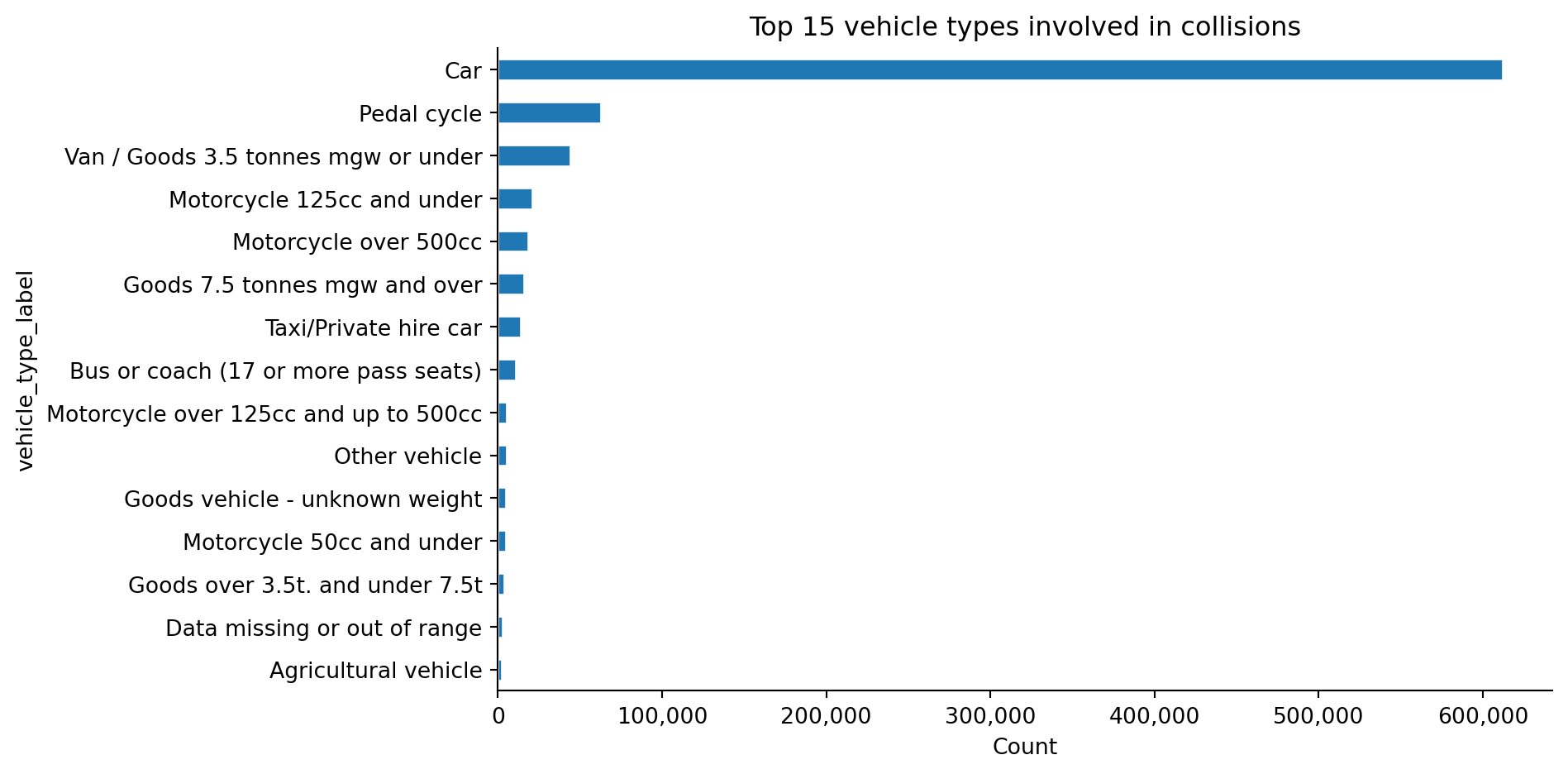
  4. How do severity, road type, time of day, and vehicle mix vary?
  5. How well do the three STATS19 tables link together?

3 What STATS19 is

STATS19 is the official Great Britain road casualty statistics dataset, published by the Department for Transport under the Road Traffic Act 1988.[^1] It records every personal-injury road collision reported to the police, split across three linked tables: collisions, vehicles involved, and casualties.

The dataset has been collected since 1926 using a standardised reporting form completed by police officers attending the scene. Since 2016, many forces have migrated to the CRASH (Collision Reporting And SHaring) system, which replaced paper forms with a structured digital workflow.[^2]

4 How the data is collected

Attending officers record structured fields covering:

  • Collision context — date, time, location (GPS), road type, junction layout, weather, lighting, surface condition.
  • Vehicles — type, manoeuvre, point of impact, driver age and sex.
  • Casualties — severity, class (driver / passenger / pedestrian), age, sex, and whether seat belt or helmet was worn.

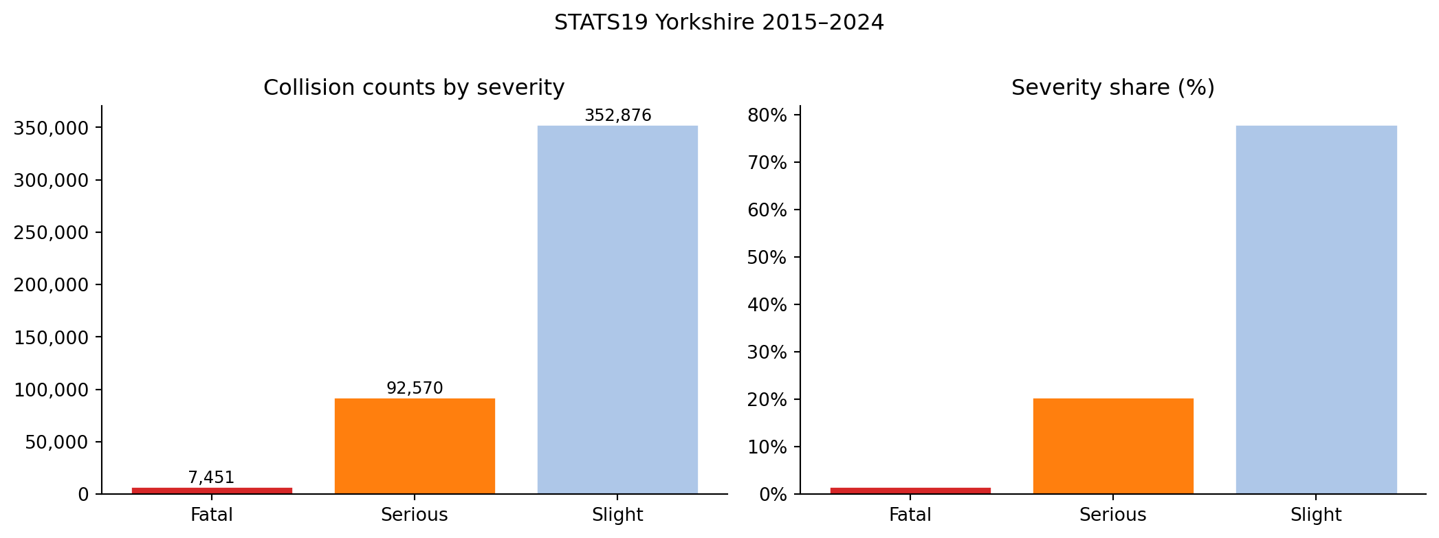
Severity is classified as Fatal (death within 30 days), Serious (injury requiring hospital attention — detained in hospital, fractures, concussion, severe cuts, etc.), or Slight (minor injury — sprains, bruises, shock).[^3]

4.1 Known reporting biases

Several biases in STATS19 are well-documented and matter for how the data is used:

  • Under-reporting of slight injuries — comparisons with hospital admissions (HES) and NTS self-report data suggest STATS19 captures roughly 60–70% of slight injuries and around 85% of serious injuries. Fatal collisions are near-complete.[^4]
  • Cyclist and pedestrian collisions are particularly under-reported when no motor vehicle is involved or when injuries are initially judged minor.
  • Severity re-grading (2016 onwards) — the switch to the CRASH system introduced injury-based severity coding, which increased the recorded count of “serious” injuries relative to pre-2016 methodology. Time-series analysis across the transition requires care.[^5]
  • Damage-only collisions are not recorded at all — STATS19 is injury-only.
WarningImplication for the model

The model learns collision risk from reported injury collisions. Areas or road types with lower reporting rates (minor rural roads, cyclist infrastructure away from motor traffic) will appear safer than they actually are. The model’s predictions should be interpreted as “expected reported injury collision rate”, not “actual collision risk”.

5 Use in practice

STATS19 is the statutory basis for:

  • DfT’s annual Reported Road Casualties Great Britain publication.[^6]
  • Local authority Road Safety Plans and junction-level safety audits.
  • Academic research into road safety — it underpins most UK-based studies of collision risk, including KSI trend analysis, speed limit evaluations, and vulnerable road user safety.

A common pattern across these uses is to combine STATS19 with traffic exposure data (AADF, WebTRIS) to produce rates rather than raw counts — which is also the approach taken in features.py.


6 Download

Source: https://www.gov.uk/government/statistical-data-sets/road-safety-open-data

Download the Last 5 years bundle for 2020–2024 and individual year files for 2015–2019. Place all CSVs in data/raw/stats19/.

Note

The file naming convention changed — files from 2019 onward use collision in the filename; earlier files use accident. The ingest module handles both.

7 Tables

File Grain Key join column
...-collision-YYYY.csv 1 row per accident accident_index
...-vehicle-YYYY.csv 1 row per vehicle involved accident_index
...-casualty-YYYY.csv 1 row per casualty accident_index

8 Key variables

8.1 Collision table

  • accident_severity — 1 Fatal, 2 Serious, 3 Slight (model target)
  • road_type, speed_limit, junction_detail
  • light_conditions, weather_conditions, road_surface_conditions
  • urban_or_rural_area
  • latitude, longitude — for spatial join to OS Open Roads / AADF

8.2 Vehicle table

  • vehicle_type — car, HGV, motorcycle, bus, etc.
  • age_of_driver, age_of_vehicle, vehicle_manoeuvre

8.3 Casualty table

  • casualty_severity, casualty_type, casualty_class

9 Setup

10 Load data

Code
from road_risk.ingest.ingest_stats19 import load_stats19, join_stats19

data       = load_stats19(raw_folder=_ROOT / "data/raw/stats19", years=YEARS)
collisions = data["collision"]
vehicles   = data["vehicle"]
casualties = data["casualty"]

df_guide = pd.read_excel(
    _ROOT / "data/raw/stats19/dft-road-casualty-statistics-road-safety-open-dataset-data-guide-2024.xlsx",
    sheet_name="2024_code_list",
)
df_guide.columns = ["table", "field_name", "code", "label", "note"]

def get_lookup(field: str) -> dict:
    rows = df_guide[df_guide["field_name"] == field].dropna(subset=["code", "label"])
    return dict(zip(rows["code"].astype(int), rows["label"]))

print(f"Collisions : {len(collisions):,} rows")
print(f"Vehicles   : {len(vehicles):,} rows")
print(f"Casualties : {len(casualties):,} rows")
Collisions : 452,897 rows
Vehicles   : 834,841 rows
Casualties : 604,874 rows

11 Missingness and data quality

Code
def missingness_report(df: pd.DataFrame, name: str) -> pd.DataFrame:
    total  = len(df)
    report = (
        df.isnull().sum()
        .rename("n_missing")
        .to_frame()
        .assign(pct_missing=lambda x: 100 * x["n_missing"] / total)
        .query("n_missing > 0")
        .sort_values("pct_missing", ascending=False)
    )
    print(f"{name}: {total:,} rows — {len(report)} columns with missing values")
    return report

miss_c = missingness_report(collisions, "Collisions")
display(miss_c.head(15))
Collisions: 452,897 rows — 6 columns with missing values
n_missing pct_missing
location_easting_osgr 103 0.023
location_northing_osgr 103 0.023
longitude 103 0.023
latitude 103 0.023
local_authority_highway_current 103 0.023
speed_limit 26 0.006
Code
bad_geo = collisions[collisions[["latitude", "longitude"]].isnull().any(axis=1)]
print(f"Collisions missing lat/lon: {len(bad_geo):,} ({100*len(bad_geo)/len(collisions):.2f}%)")

# Yorkshire bounding box check
in_bbox = (
    collisions["latitude"].between(53.30, 54.60) &
    collisions["longitude"].between(-2.20, -0.08)
)
out_bbox = collisions[
    collisions[["latitude","longitude"]].notna().all(axis=1) & ~in_bbox
]
print(f"Valid coords outside Yorkshire bbox: {len(out_bbox):,}")

print("\nSpeed limit distribution:")
print(collisions["speed_limit"].value_counts().sort_index().to_string())
Collisions missing lat/lon: 103 (0.02%)
Valid coords outside Yorkshire bbox: 329,462

Speed limit distribution:
speed_limit
-1.000         6
20.000     19398
30.000    282139
40.000     40392
50.000     19577
60.000     64048
70.000     27311

12 Collision severity

12.1 Overall distribution

Code
counts = collisions["severity_label"].value_counts().reindex(["Fatal", "Serious", "Slight"])
props  = counts / counts.sum() * 100
colours = [SEVERITY_COLOURS[s] for s in counts.index]

fig, axes = plt.subplots(1, 2, figsize=(11, 4))

bars = axes[0].bar(counts.index, counts.values, color=colours, edgecolor="white")
axes[0].set_title("Collision counts by severity")
axes[0].set_xlabel("")
axes[0].tick_params(axis="x", rotation=0)
axes[0].yaxis.set_major_formatter(mticker.FuncFormatter(lambda x, _: f"{int(x):,}"))
axes[0].spines[["top", "right"]].set_visible(False)
for bar in bars:
    axes[0].text(bar.get_x() + bar.get_width()/2, bar.get_height() + 50,
                 f"{int(bar.get_height()):,}", ha="center", va="bottom", fontsize=9)

axes[1].bar(props.index, props.values, color=colours, edgecolor="white")
axes[1].set_title("Severity share (%)")
axes[1].set_xlabel("")
axes[1].yaxis.set_major_formatter(mticker.PercentFormatter())
axes[1].tick_params(axis="x", rotation=0)
axes[1].spines[["top", "right"]].set_visible(False)

plt.suptitle("STATS19 Yorkshire 2015–2024", y=1.01)
plt.tight_layout()
plt.show()
Figure 1: Collision counts and share by severity — Yorkshire 2015–2024

12.2 By road type

Code
sev_road = (
    collisions.groupby(["road_type_label", "severity_label"])
    .size()
    .unstack(fill_value=0)
    .reindex(columns=["Fatal", "Serious", "Slight"])
)
sev_road_pct = sev_road.div(sev_road.sum(axis=1), axis=0) * 100

colours_list = [SEVERITY_COLOURS[c] for c in ["Fatal", "Serious", "Slight"]]
fig, axes = plt.subplots(1, 2, figsize=(14, 4))

sev_road.plot(kind="bar", stacked=True, ax=axes[0],
              color=colours_list, edgecolor="white", legend=False)
axes[0].set_title("Counts")
axes[0].set_xlabel("")
axes[0].set_ylabel("Collisions")
axes[0].tick_params(axis="x", rotation=30)
axes[0].yaxis.set_major_formatter(mticker.FuncFormatter(lambda x, _: f"{int(x):,}"))
axes[0].spines[["top", "right"]].set_visible(False)

sev_road_pct.plot(kind="bar", stacked=True, ax=axes[1],
                  color=colours_list, edgecolor="white")
axes[1].set_title("Share (%)")
axes[1].set_xlabel("")
axes[1].set_ylabel("%")
axes[1].tick_params(axis="x", rotation=30)
axes[1].yaxis.set_major_formatter(mticker.PercentFormatter())
axes[1].legend(title="Severity", bbox_to_anchor=(1.01, 1))
axes[1].spines[["top", "right"]].set_visible(False)

plt.suptitle("Severity by road type", y=1.01)
plt.tight_layout()
plt.show()
Figure 2: Severity distribution by road type — counts (left) and % share (right)

12.3 By speed limit

Code
sev_speed = (
    collisions.groupby(["speed_limit", "severity_label"])
    .size()
    .unstack(fill_value=0)
    .reindex(columns=["Fatal", "Serious", "Slight"])
)
total       = sev_speed.sum(axis=1)
fatal_rate  = sev_speed["Fatal"]   / total * 100
serious_rate = sev_speed["Serious"] / total * 100
slight_rate  = sev_speed["Slight"]  / total * 100

fig, ax = plt.subplots(figsize=(10, 4))
axR = ax.twinx()

ax.bar(fatal_rate.index, fatal_rate.values,
       color="#d62728", edgecolor="white", width=7, label="% Fatal")
axR.bar(serious_rate.index, serious_rate.values,
        color="none", edgecolor="black", hatch="//", width=7, label="% Serious")
axR.plot(slight_rate.index, slight_rate.values,
         color="black", linestyle="--", marker="o", label="% Slight")

ax.set_title("Collision severity rate by speed limit")
ax.set_xlabel("Speed limit (mph)")
ax.set_ylabel("% Fatal")
axR.set_ylabel("% Serious / % Slight")
ax.spines[["top"]].set_visible(False)
ax.legend(loc="upper left")
axR.legend(loc="upper right")
plt.tight_layout()
plt.show()
Figure 3: Fatal, serious, and slight rates by speed limit

13 Temporal trends

COVID years (2020–2021) are highlighted throughout.

13.1 Year-on-year

Code
yearly = collisions.groupby("year").size().reset_index(name="n_collisions")
yearly["is_covid"] = yearly["year"].isin(COVID_YEARS)

cond_ksi    = collisions["severity_label"].isin(["Fatal", "Serious"])
yearly_ksi  = collisions[cond_ksi].groupby("year").size().reset_index(name="n_ksi")

fig, ax = plt.subplots(figsize=(10, 4))
axR = ax.twinx()

colours = ["#ff7f0e" if covid else "#1f77b4" for covid in yearly["is_covid"]]
ax.bar(yearly["year"], yearly["n_collisions"], color=colours, edgecolor="white")
axR.plot(yearly_ksi["year"], yearly_ksi["n_ksi"],
         color="black", marker="o", linewidth=1.8, label="KSI")

ax.set_title("Collisions per year — Yorkshire")
ax.set_xlabel("Year")
ax.set_ylabel("All collisions")
axR.set_ylabel("Killed or seriously injured")
ax.yaxis.set_major_formatter(mticker.FuncFormatter(lambda x, _: f"{int(x):,}"))
axR.set_ylim(0, yearly_ksi["n_ksi"].max() * 1.2)
ax.spines[["top"]].set_visible(False)

from matplotlib.patches import Patch
ax.legend(handles=[
    Patch(color="#1f77b4", label="Normal"),
    Patch(color="#ff7f0e", label="COVID"),
], loc="upper left")
axR.legend(loc="lower right")
plt.tight_layout()
plt.show()
Figure 4: Collisions per year with serious/fatal overlay

13.2 Monthly seasonality

Code
monthly = (
    collisions[~collisions["year"].isin(COVID_YEARS)]
    .groupby("month")
    .size()
    .reset_index(name="n_collisions")
)
month_names = ["Jan","Feb","Mar","Apr","May","Jun","Jul","Aug","Sep","Oct","Nov","Dec"]

fig, ax = plt.subplots(figsize=(10, 4))
ax.plot(monthly["month"], monthly["n_collisions"], marker="o", linewidth=2, color="#1f77b4")
ax.set_xticks(range(1, 13))
ax.set_xticklabels(month_names)
ax.set_title("Monthly collision pattern (pre/post COVID years only)")
ax.set_ylabel("Total collisions 2015–2024 (excl. 2020–21)")
ax.yaxis.set_major_formatter(mticker.FuncFormatter(lambda x, _: f"{int(x):,}"))
ax.spines[["top", "right"]].set_visible(False)
plt.tight_layout()
plt.show()
Figure 5: Monthly collision pattern (COVID years excluded)

13.3 Day of week

Code
dow_order = ["Monday","Tuesday","Wednesday","Thursday","Friday","Saturday","Sunday"]
dow = (
    collisions[~collisions["year"].isin(COVID_YEARS)]
    .groupby("day_name")
    .size()
    .reindex(dow_order)
)

fig, ax = plt.subplots(figsize=(10, 4))
ax.bar(dow.index, dow.values, color="#1f77b4", edgecolor="white")
ax.set_title("Collisions by day of week (excl. COVID years)")
ax.set_ylabel("Total collisions")
ax.yaxis.set_major_formatter(mticker.FuncFormatter(lambda x, _: f"{int(x):,}"))
ax.spines[["top", "right"]].set_visible(False)
plt.tight_layout()
plt.show()
Figure 6: Collisions by day of week (COVID years excluded)

13.4 Hour of day

Code
if collisions["hour"].notna().sum() > 0:
    hourly = (
        collisions[~collisions["year"].isin(COVID_YEARS)]
        .groupby(["hour", "severity_label"])
        .size()
        .unstack(fill_value=0)
        .reindex(columns=["Fatal", "Serious", "Slight"])
    )

    fig, ax = plt.subplots(figsize=(12, 4))
    axR = ax.twinx()

    ax.plot(hourly.index, hourly["Slight"],
            color="#aec7e8", linewidth=2, marker=".", label="Slight")
    axR.plot(hourly.index, hourly["Serious"],
             color="#ff7f0e", linewidth=1.8, linestyle="--", marker="o", label="Serious")
    axR.plot(hourly.index, hourly["Fatal"],
             color="#d62728", linewidth=1.8, linestyle="-.", marker="s", label="Fatal")

    ax.set_title("Collisions by hour of day and severity (excl. COVID years)")
    ax.set_xlabel("Hour of day")
    ax.set_ylabel("Slight collisions")
    axR.set_ylabel("Serious / Fatal collisions")
    ax.set_xticks(range(0, 24))
    ax.spines[["top"]].set_visible(False)

    lines  = ax.get_lines() + axR.get_lines()
    labels = [l.get_label() for l in lines]
    ax.legend(lines, labels, fontsize=8, loc="upper left")
    plt.tight_layout()
    plt.show()
else:
    print("No time data available — check 'time' column name.")
Figure 7: Collisions by hour of day and severity (COVID years excluded)

14 Vehicle types

14.1 Distribution

Code
vtype_counts = vehicles["vehicle_type_label"].value_counts().head(15)

fig, ax = plt.subplots(figsize=(10, 5))
vtype_counts.plot(kind="barh", ax=ax, color="#1f77b4", edgecolor="white")
ax.set_title("Top 15 vehicle types involved in collisions")
ax.set_xlabel("Count")
ax.invert_yaxis()
ax.xaxis.set_major_formatter(mticker.FuncFormatter(lambda x, _: f"{int(x):,}"))
ax.spines[["top", "right"]].set_visible(False)
plt.tight_layout()
plt.show()
Figure 8: Top 15 vehicle types involved in collisions

14.2 HGV involvement by road type

Code
# Vehicle type codes from data guide — verify against get_lookup("vehicle_type")
HGV_TYPES = [3, 11, 20, 21, 98]

veh_with_road = vehicles.merge(
    collisions[["collision_index", "road_type_label", "collision_severity"]],
    on="collision_index", how="left"
)
veh_with_road["is_hgv"] = veh_with_road["vehicle_type"].isin(HGV_TYPES)

hgv_by_road = (
    veh_with_road.groupby("road_type_label")["is_hgv"]
    .agg(hgv_count="sum", total="count")
    .assign(hgv_pct=lambda x: 100 * x["hgv_count"] / x["total"])
    .sort_values("hgv_pct", ascending=False)
)
display(hgv_by_road)
hgv_count total hgv_pct
road_type_label
Dual carriageway 12996 134849 9.637
Slip road 691 9874 6.998
One way street 707 10136 6.975
Roundabout 3506 51023 6.871
Single carriageway 38344 623485 6.150
Unknown 322 5474 5.882
Note

HGV vehicle type codes (3, 11, 20, 21, 98) are approximate — verify against get_lookup("vehicle_type") before using in the model.

14.3 Vehicles per collision

Code
veh_per_collision = vehicles.groupby("collision_index").size()
print(f"Vehicles per collision — mean: {veh_per_collision.mean():.2f}, max: {veh_per_collision.max()}")

fig, ax = plt.subplots(figsize=(8, 4))
veh_per_collision.value_counts().sort_index().head(8).plot(
    kind="bar", ax=ax, color="#1f77b4", edgecolor="white"
)
ax.set_title("Number of vehicles per collision")
ax.set_xlabel("Vehicles involved")
ax.set_ylabel("Number of collisions")
ax.tick_params(axis="x", rotation=0)
ax.yaxis.set_major_formatter(mticker.FuncFormatter(lambda x, _: f"{int(x):,}"))
ax.spines[["top", "right"]].set_visible(False)
plt.tight_layout()
plt.show()
Vehicles per collision — mean: 1.84, max: 16
Figure 9: Number of vehicles involved per collision

15 Geography

Code
import geopandas as gpd
import contextily as cx
import numpy as np
import matplotlib.pyplot as plt
import matplotlib.colors as mcolors

# Filter to valid coords within Yorkshire bbox
valid = (
    collisions["latitude"].between(53.30, 54.60) &
    collisions["longitude"].between(-2.20, -0.08) &
    collisions["latitude"].notna() &
    collisions["longitude"].notna()
)
cols_geo = collisions[valid].copy()

gdf = gpd.GeoDataFrame(
    cols_geo,
    geometry=gpd.points_from_xy(cols_geo["longitude"], cols_geo["latitude"]),
    crs="EPSG:4326",
).to_crs(epsg=3857)

severities = ["Slight", "Serious", "Fatal"]
cmaps      = ["Blues",  "Oranges", "Reds"]
# gridsize controls resolution — lower = coarser, faster
GRIDSIZE = 200

# Shared spatial extent
minx, miny, maxx, maxy = gdf.total_bounds
pad = max(maxx - minx, maxy - miny) * 0.03
extent = (minx - pad, maxx + pad, miny - pad, maxy + pad)

fig, axes = plt.subplots(1, 3, figsize=(15, 7))

for ax, sev, cmap in zip(axes, severities, cmaps):
    sub = gdf[gdf["severity_label"] == sev]
    x, y = sub.geometry.x.values, sub.geometry.y.values

    # 2D histogram binned to grid
    h, xedges, yedges = np.histogram2d(
        x, y, bins=GRIDSIZE,
        range=[[extent[0], extent[1]], [extent[2], extent[3]]],
    )
    h = np.ma.masked_where(h == 0, h)   # transparent empty cells

    ax.set_xlim(extent[0], extent[1])
    ax.set_ylim(extent[2], extent[3])

    try:
        cx.add_basemap(ax, source=cx.providers.CartoDB.Positron,
                       zoom="auto", attribution_size=5)
    except Exception as exc:
        print(f"Basemap unavailable: {exc}")

    ax.pcolormesh(
        xedges, yedges, h.T,
        cmap=cmap,
        norm=mcolors.PowerNorm(gamma=0.4),  # compress high-count cells
        alpha=0.75,
        zorder=2,
    )

    ax.set_axis_off()
    ax.set_title(f"{sev}  (n={len(sub):,})", fontsize=11)

fig.suptitle("Collision density — Yorkshire 2015–2024", fontsize=13, y=1.01)
plt.tight_layout()
plt.show()
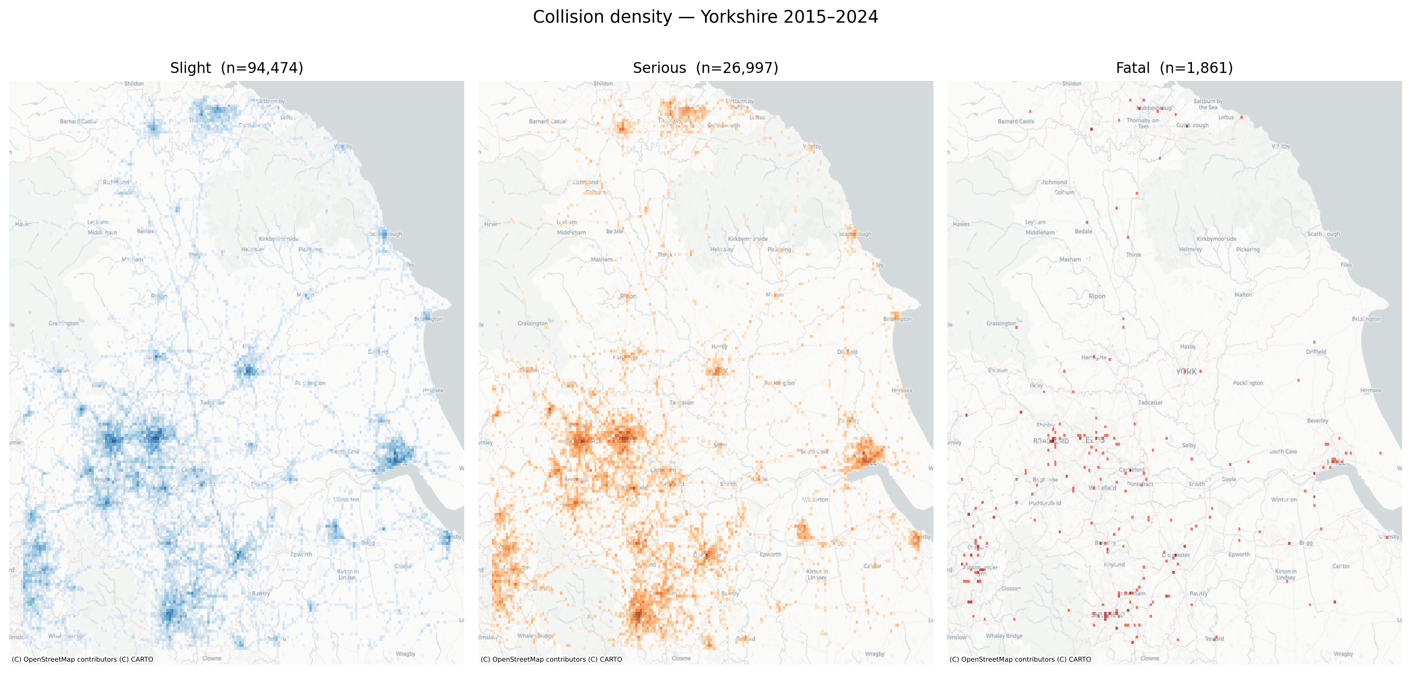
Figure 10: Collision density by severity — Yorkshire 2015–2024 (COVID years included)

16 Join quality

Code
collision_ids = set(collisions["collision_index"])
vehicle_ids   = set(vehicles["collision_index"])
casualty_ids  = set(casualties["collision_index"])

print("=== Join coverage ===")
print(f"Collision IDs                     : {len(collision_ids):,}")
print()
print(f"Vehicle records                   : {len(vehicles):,}")
print(f"  matched to a collision          : {len(vehicle_ids & collision_ids):,}"
      f"  ({100*len(vehicle_ids & collision_ids)/len(vehicle_ids):.1f}%)")
print(f"  orphaned (no collision match)   : {len(vehicle_ids - collision_ids):,}")
print()
print(f"Casualty records                  : {len(casualties):,}")
print(f"  matched to a collision          : {len(casualty_ids & collision_ids):,}"
      f"  ({100*len(casualty_ids & collision_ids)/len(casualties):.1f}%)")
print(f"  orphaned (no collision match)   : {len(casualty_ids - collision_ids):,}")
print()
print(f"Collisions with no vehicles       : {len(collision_ids - vehicle_ids):,}")
print(f"Collisions with no casualties     : {len(collision_ids - casualty_ids):,}")
=== Join coverage ===
Collision IDs                     : 452,897

Vehicle records                   : 834,841
  matched to a collision          : 452,897  (100.0%)
  orphaned (no collision match)   : 0

Casualty records                  : 604,874
  matched to a collision          : 452,897  (74.9%)
  orphaned (no collision match)   : 0

Collisions with no vehicles       : 0
Collisions with no casualties     : 0
Code
joined = join_stats19(data)
print(f"Joined table : {len(joined):,} rows × {joined.shape[1]} cols")
print(f"Casualties   : {len(casualties):,}")
print(f"Ratio        : {len(joined)/len(casualties):.3f}  (should be ~1.0)")

dup_cols = [c for c in joined.columns if joined.columns.tolist().count(c) > 1]
print(f"\nDuplicate columns after join: {dup_cols if dup_cols else 'none ✓'}")

key_cols = ["collision_index", "collision_severity", "vehicle_type",
            "casualty_severity", "casualty_type"]
print("\nNull rates on key joined columns:")
for col in key_cols:
    if col in joined.columns:
        n_null = joined[col].isnull().sum()
        print(f"  {col:35s}: {n_null:,} ({100*n_null/len(joined):.1f}%)")
Joined table : 1,173,293 rows × 104 cols
Casualties   : 604,874
Ratio        : 1.940  (should be ~1.0)

Duplicate columns after join: none ✓

Null rates on key joined columns:
  collision_index                    : 0 (0.0%)
  collision_severity                 : 0 (0.0%)
  vehicle_type                       : 0 (0.0%)
  casualty_severity                  : 0 (0.0%)
  casualty_type                      : 0 (0.0%)

17 Notes for clean.py

Fill in after running:

  • Missing lat/lon — rows to drop
  • Out-of-bbox coordinates — rows to investigate
  • Speed limit outliers — values to recode as null
  • HGV vehicle type codes — confirm codes from data guide
  • COVID flag — years 2020–2021 to be flagged in features.py
  • Join orphans — vehicle / casualty records unmatched — investigate

18 Known issues

  • junction_detail had an error corrected in the November 2025 release — ensure you download the latest versions of all files.
  • 2020–2021 volumes are substantially lower due to COVID lockdowns.
  • A small number of records have missing or implausible lat/lon — these are dropped in clean.py.

Open Road Risk


Built with Quarto