import os
import logging
from pathlib import Path
import numpy as np
import pandas as pd
import matplotlib.pyplot as plt
import seaborn as sns

from road_risk.config import _ROOT as ROOT
from road_risk.model.constants import MONTH_ORDER

# Configure paths
WEBTRIS_RAW = ROOT / "data/raw/webtris"
WEBTRIS_CLEAN = ROOT / "data/processed/webtris/webtris_clean.parquet"
TEMPORAL_PROFILES = ROOT / "data/models/temporal_profiles.parquet"

sns.set_theme(style="whitegrid")Temporal Traffic Exploration: Seasonality and Day-of-Week Patterns
Exploratory analysis of traffic seasonality, day-of-week patterns, temporal variation, and implications for exposure modelling.
Overview
This notebook explores the temporal dimensions of traffic flow using WebTRIS sensor data. We analyze how traffic volumes and compositions change across different months and between weekdays and weekends.
The goal is to determine which temporal patterns are link-specific (requiring granular modelling) and which are stable enough to be treated as global constants.
We investigate: 1. Monthly Seasonality: High-season vs. low-season flow amplitudes. 2. Weekday/Weekend Ratios: Commuter-heavy vs. leisure-heavy road signatures. 3. Time-of-Day Intensity: The ratio of daytime to nighttime flow. 4. HGV Mixing: How vehicle composition shifts across these same axes.
1 Variance Analysis (Weekday/Weekend)
We begin by testing the variance of the weekday/weekend ratio at the individual sensor level. If the ratio is stable across different sites within the same month, it suggests the pattern is universal rather than link-specific.
We start with the strongest test: whether different sensors in the same month give similar weekday/weekend ratios. If they do, the descriptor has no link-specific variation to model.
# Load a larger sample of raw parquets to test variance
files = [f for f in os.listdir(WEBTRIS_RAW) if "2023" in f and f.endswith(".parquet")]
df_list = []
for file in files:
    df = pd.read_parquet(WEBTRIS_RAW / file, columns=["site_id", "monthname", "adt24hour", "awt24hour"])
    df_list.append(df)

raw_2023 = pd.concat(df_list, ignore_index=True)
raw_2023["adt24hour"] = pd.to_numeric(raw_2023["adt24hour"], errors="coerce")
raw_2023["awt24hour"] = pd.to_numeric(raw_2023["awt24hour"], errors="coerce")
raw_2023["ww_ratio"] = raw_2023["awt24hour"] / raw_2023["adt24hour"].replace(0, np.nan)

# Calculate within-month standard deviation across sites
month_stats = raw_2023.groupby("monthname")["ww_ratio"].agg(["mean", "std", "count"])
print("Per-site Weekday/Weekend Ratio stats by month:")
print(month_stats.round(4))

overall_std = raw_2023.groupby("monthname")["ww_ratio"].std().mean()
print(f"\nAverage within-month standard deviation across sites: {overall_std:.3f}")
Per-site Weekday/Weekend Ratio stats by month:
mean std count
monthname
Apr 1.0869 0.0379 3631
Aug 1.0483 0.0289 3579
Dec 1.0760 0.0378 4240
Feb 1.0706 0.0331 4536
Jan 1.0896 0.0325 4550
Jul 1.0597 0.0439 3638
Jun 1.0579 0.0322 3638
Mar 1.0632 0.0279 4529
May 1.0593 0.0277 3631
Nov 1.0667 0.0298 4249
Oct 1.0493 0.0304 4363
Sep 1.0533 0.0335 4316
Average within-month standard deviation across sites: 0.0331.1 Interpretation
The data shows that the standard deviation across sites within any given month is consistently ~0.03. This low variance suggests that individual roads do not deviate significantly from the network-wide weekday/weekend behavior.
2 Monthly Seasonality Analysis
We now switch to the temporal_profiles.parquet, which aggregates data at the road corridor grain and calculates seasonal indices.
profiles = pd.read_parquet(TEMPORAL_PROFILES)
profiles = profiles[profiles["n_site_months"] > 0].copy()

# Broad classification
profiles['road_type'] = profiles['road_prefix'].apply(
    lambda x: 'Motorway' if str(x).startswith('M') else ('A-Road' if str(x).startswith('A') else 'Other')
)

# Ensure chronological sorting
profiles["monthname"] = pd.Categorical(profiles["monthname"], categories=MONTH_ORDER, ordered=True)

profiles.sample(5)| road_prefix | monthname | month_num | mean_adt24 | mean_awt24 | mean_large_pct | n_site_months | seasonal_index | weekday_weekend_ratio | road_type | |
|---|---|---|---|---|---|---|---|---|---|---|
| 121378 | A1M/ | Nov | 11 | 29919.729362 | 32126.707109 | 22.352468 | 2350 | 0.993242 | 1.073763 | A-Road |
| 64799 | 8304 | Dec | 12 | 8536.214286 | 9047.428571 | 11.807143 | 14 | 0.953909 | 1.059888 | Other |
| 97487 | 9356 | Dec | 12 | 22041.666667 | 24309.333333 | 9.500000 | 3 | 0.926697 | 1.102881 | Other |
| 11546 | 6516 | Mar | 3 | 24028.000000 | 26439.000000 | 21.900000 | 1 | 0.976961 | 1.100341 | Other |
| 81844 | 9010 | May | 5 | 32062.000000 | 32908.000000 | 6.633333 | 3 | 1.044752 | 1.026386 | Other |
2.1 Seasonal Index Distribution
The seasonal index is the monthly flow divided by the annual average. We want to see if different road types have different seasonal “signatures.”
fig, ax = plt.subplots(figsize=(12, 6))

sns.lineplot(
    data=profiles,
    x="monthname",
    y="seasonal_index",
    hue="road_type",
    marker="o",
    errorbar=("sd", 1),
    ax=ax
)

ax.axhline(1.0, color="black", linestyle="--", alpha=0.5)
ax.set_title("Seasonal Traffic Index by Road Type (Mean ± 1 SD)")
ax.set_ylabel("Seasonal Index (1.0 = Annual Average)")
plt.show()

print("Mean Seasonal Index by Month and Road Type:")
print(profiles.groupby(["monthname", "road_type"], observed=True)["seasonal_index"].mean().unstack().round(3))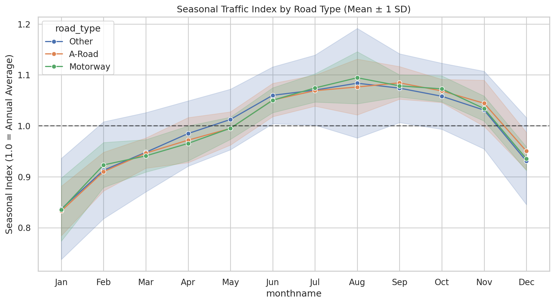
Mean Seasonal Index by Month and Road Type:
road_type  A-Road  Motorway  Other
monthname
Jan         0.833     0.835  0.837
Feb         0.910     0.923  0.913
Mar         0.947     0.941  0.948
Apr         0.972     0.965  0.985
May         0.995     0.995  1.013
Jun         1.051     1.050  1.060
Jul         1.069     1.074  1.070
Aug         1.076     1.094  1.084
Sep         1.084     1.079  1.074
Oct         1.069     1.073  1.058
Nov         1.044     1.034  1.031
Dec         0.950     0.935  0.931
2.2 Interpretation
- Amplitude: The vertical distance between the summer peak and winter trough shows a significant ~30% seasonal swing.
- Convergence: The lines for Motorways and A-Roads overlap closely, with seasonal indices sitting within ±0.02 of each other in every month. This means seasonality is a global phenomenon rather than a link-specific one.
3 Weekday vs. Weekend Profiles
We investigate the stability of the weekday/weekend ratio across the network.
The Variance Analysis section used raw 2023 chunks at site grain. This section uses the corridor-level aggregations from temporal_profiles.parquet, confirming the same result holds at corridor grain.
fig, (ax1, ax2) = plt.subplots(1, 2, figsize=(16, 6))

# Distribution across all sites/months
sns.histplot(profiles["weekday_weekend_ratio"].dropna(), bins=40, kde=True, color="seagreen", ax=ax1)
ax1.axvline(profiles["weekday_weekend_ratio"].median(), color="red", linestyle="--")
ax1.set_title("Distribution of Weekday/Weekend Ratios")
ax1.set_xlabel("Ratio (AWT / ADT)")

# Stability by month
sns.boxplot(data=profiles, x="monthname", y="weekday_weekend_ratio", color="lightblue", ax=ax2)
ax2.axhline(1.0, color="black", linestyle="--", alpha=0.3)
ax2.set_title("Ratio Stability Across Months")
ax2.set_ylabel("Weekday/Weekend Ratio")

plt.tight_layout()
plt.show()

# Mean check by road type
print("Mean Weekday/Weekend Ratio by Road Type:")
print(profiles.groupby("road_type")["weekday_weekend_ratio"].mean().round(4))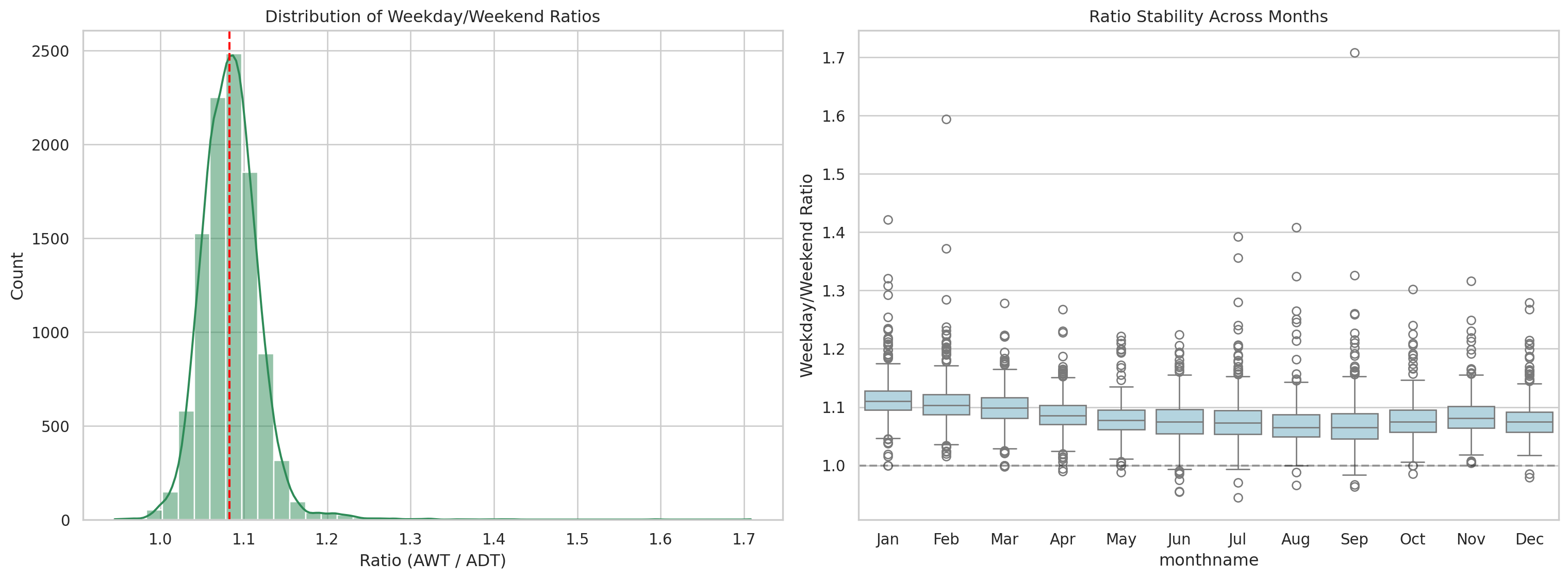
Mean Weekday/Weekend Ratio by Road Type:
road_type
A-Road      1.0779
Motorway    1.0712
Other       1.0849
Name: weekday_weekend_ratio, dtype: float64
3.1 Interpretation
Mean ratio is 1.08; standard deviation across sites within any month is ~0.03; mean is essentially identical across road types (motorway 1.073, A-road 1.076, other 1.085). The descriptor has no link-specific variation to model.
4 Time-of-Day Intensity (Day vs. Night)
Using the webtris_clean.parquet dataset, we examine the core_overnight_ratio. This measures the daytime flow per hour relative to the nighttime flow per hour.
webtris_clean = pd.read_parquet(WEBTRIS_CLEAN)
site_tod = webtris_clean.groupby("site_id")["core_overnight_ratio"].mean().dropna()

fig, ax = plt.subplots(figsize=(10, 5))
sns.histplot(site_tod, bins=50, kde=True, color="purple", ax=ax)
ax.set_title("Daytime-to-Nighttime Intensity Ratio")
ax.set_xlabel("Ratio (Mean Day Flow / Mean Night Flow)")
plt.show()

print(f"5th Percentile: {site_tod.quantile(0.05):.2f}")
print(f"95th Percentile: {site_tod.quantile(0.95):.2f}")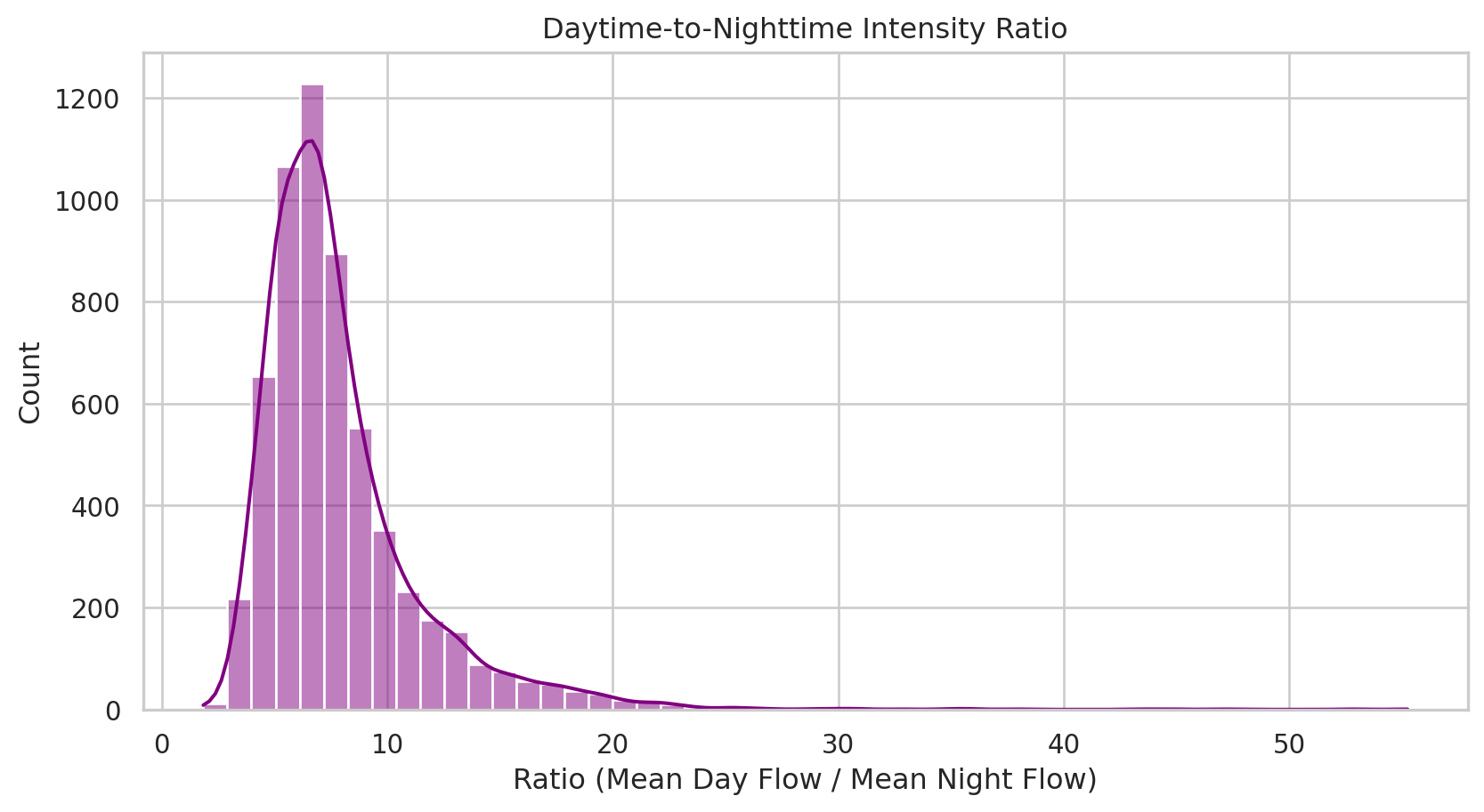
5th Percentile: 4.13
95th Percentile: 14.91
4.1 Interpretation
Unlike the weekday/weekend ratio, this distribution is wide, spanning from 4.2 to 15.2. This indicates that time-of-day behavior is highly link-specific. Some roads carry substantial overnight flows (e.g., freight corridors), while others are almost exclusively used during the day.
5 Heavy Goods Vehicle (HGV) Composition
Finally, we look at how the large vehicle percentage fluctuates across the network.
fig, ax = plt.subplots(figsize=(12, 6))

sns.boxplot(data=profiles, x="monthname", y="mean_large_pct", hue="road_type", ax=ax)
ax.set_title("Large Vehicle Percentage by Month and Road Type")
ax.set_ylabel("HGV %")
plt.legend(bbox_to_anchor=(1.05, 1), loc='upper left')
plt.show()

print("Mean Large Vehicle Percentage by Month and Road Type:")
print(profiles.groupby(["monthname", "road_type"], observed=True)["mean_large_pct"].mean().unstack().round(2))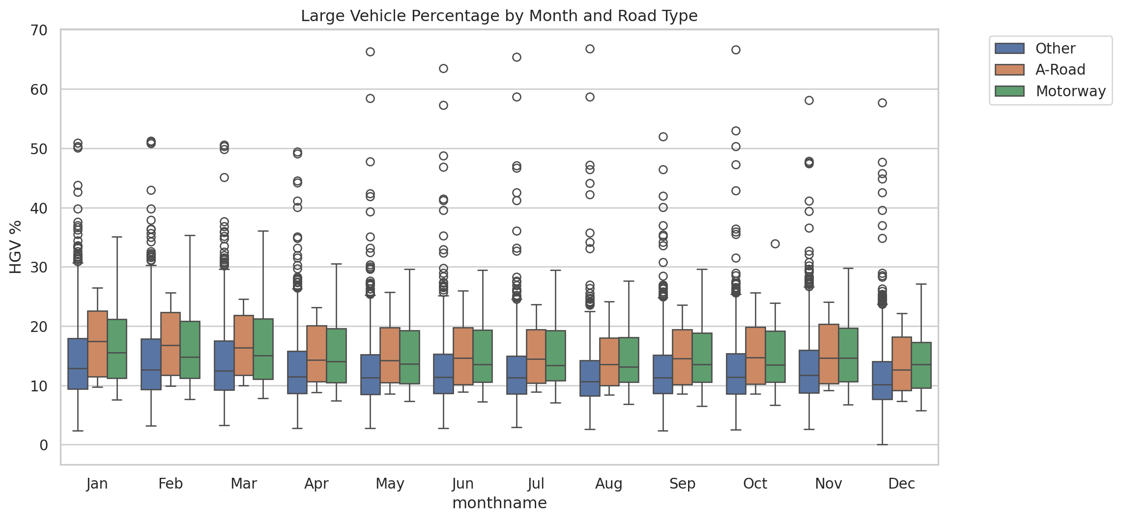
Mean Large Vehicle Percentage by Month and Road Type:
road_type  A-Road  Motorway  Other
monthname
Jan         17.51     17.10  14.41
Feb         17.26     16.83  14.22
Mar         17.05     16.76  13.98
Apr         15.63     15.34  12.97
May         15.55     15.12  12.65
Jun         15.49     15.08  12.72
Jul         15.16     15.03  12.50
Aug         14.37     14.26  11.88
Sep         14.98     14.86  12.57
Oct         15.45     15.34  12.69
Nov         15.69     15.69  13.14
Dec         13.89     13.86  11.55
5.1 Interpretation
HGV percentage shows a ~3pp summer dip across all road types. This is largely a denominator artefact — total traffic rises ~30% in summer while HGV volumes stay roughly flat — not a freight-side seasonal pattern. The within-road-class spread visible in the boxplot is genuine variation in road character, but a cleaner descriptor would be HGV volume (vehicles/day) rather than HGV percentage. Per-site within-month std check still warranted before drawing a verdict; if HGV is eventually taken to ablation, volume is the better feature. Worth a per-site within-month std analysis matching the Variance Analysis section before drawing a final verdict.
6 Data Depth Check
We verify the amount of data backing these observations to ensure statistical confidence.
# Site counts per corridor
site_counts = profiles.groupby("road_prefix")["n_site_months"].sum() / 12
print(f"Total Unique Corridors: {len(site_counts)}")

fig, ax = plt.subplots(figsize=(10, 4))
sns.histplot(site_counts, bins=30, log_scale=(True, False), ax=ax)
ax.set_title("Distribution of Sites per Corridor (Log Scale)")
ax.set_xlabel("Approximate Sites")
plt.show()
Total Unique Corridors: 879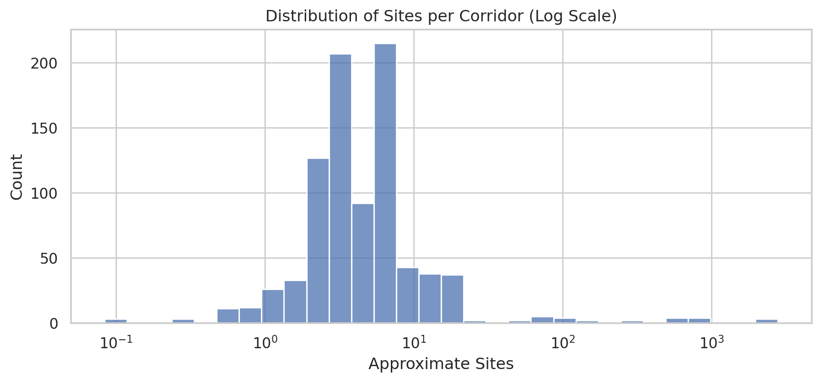
7 Summary of Potential Modelling Implications
Based on the variance observed in the plots above:
| Dimension | Observed Variance | Modelling Strategy |
|---|---|---|
| Monthly Seasonality | High amplitude, low inter-link variance. | Handle via global monthly multipliers. |
| Weekday vs. Weekend | Low variance across network (~1.08). | Treat as a global constant. |
| Time-of-Day | High inter-link variance (4.2 - 15.2). | Treat as link-specific (Priority for ablation). |
| HGV Mix | Global seasonal swing (~3pp) and substantial within-class spread. | Status: not formally tested at site grain. May carry signal beyond road class. |