Exploratory analysis of traffic volume data, AADF patterns, WebTRIS observations, exposure distributions, and model inputs.
1 Overview
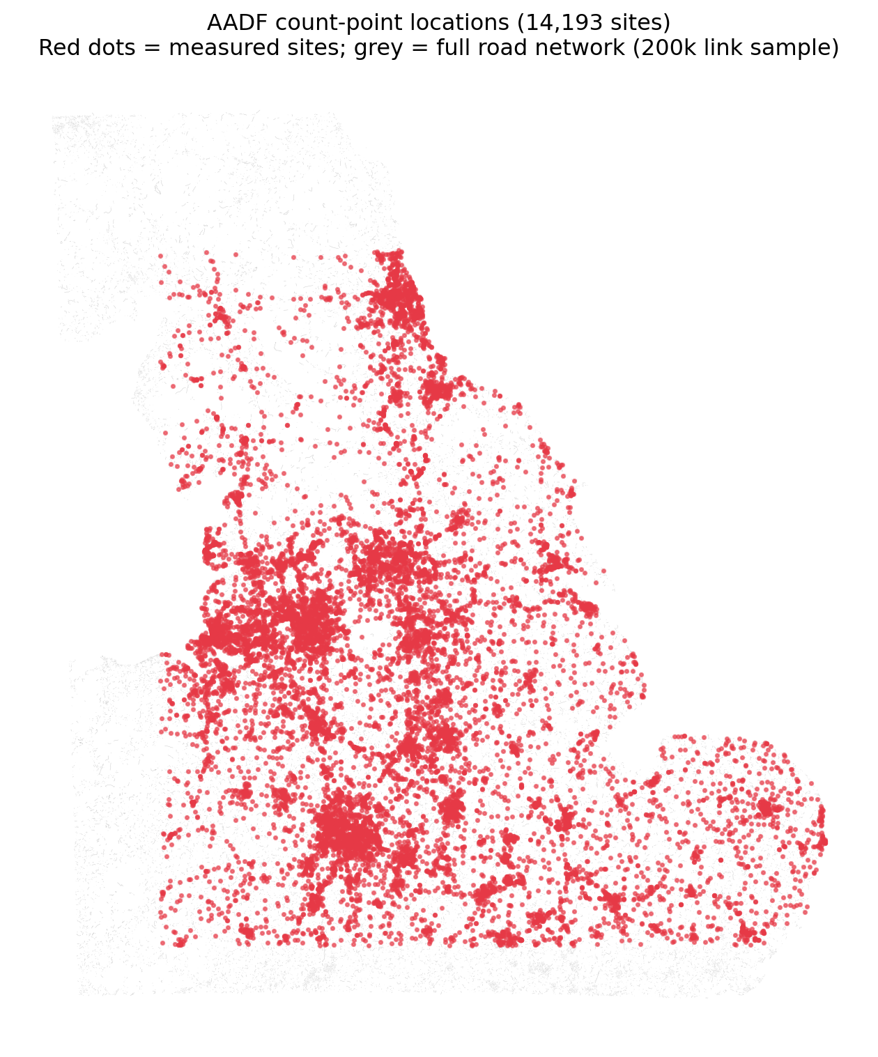
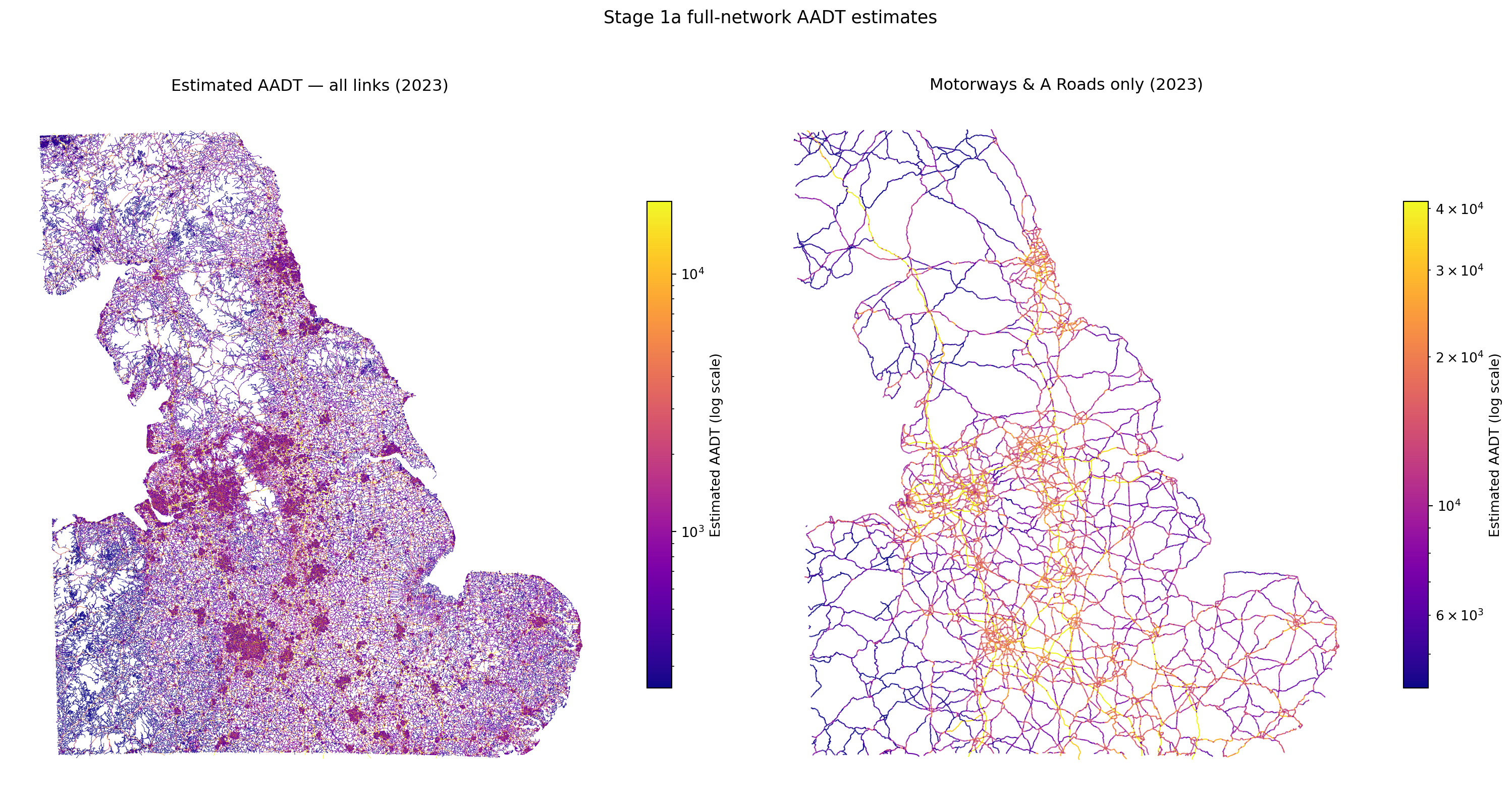
Stage 1a estimates Annual Average Daily Traffic (AADT) for every OS Open Roads link in the study area. Directly measured AADF count points cover only a minority of road links — particularly minor and unclassified roads — so a gradient-boosted regressor is trained on those measured points and applied to the full 2.1M-link network.
This page covers:
The measured AADF count-point data used for training
How the model was built and validated
The resulting full-network AADT estimates and their geographic pattern
from pathlib import Pathimport jsonimport numpy as npimport pandas as pdimport matplotlib.pyplot as pltimport matplotlib.colors as mcolorsfrom road_risk.config import _ROOT as ROOTRANDOM_STATE =42try:import geopandas as gpd HAS_GPD =TrueexceptException: HAS_GPD =Falseaadf = pd.read_parquet(ROOT /"data/processed/aadf/aadf_clean.parquet")aadt_path = ROOT /"data/models/aadt_estimates.parquet"aadt = pd.read_parquet(aadt_path) if aadt_path.exists() else pd.DataFrame()if HAS_GPD: or_path = ROOT /"data/processed/shapefiles/openroads.parquet" openroads = gpd.read_parquet(or_path) if or_path.exists() elseNoneelse: openroads =Noneval_path = ROOT /"data/models/aadt_validation_summary.parquet"val_summary = pd.read_parquet(val_path) if val_path.exists() else pd.DataFrame()print(f"AADF count points : {aadf['count_point_id'].nunique():,} count points × {aadf['year'].nunique()} years ({aadf.shape[0]:,} rows)")print(f"AADT estimates : {aadt['link_id'].nunique():,} links × {aadt['year'].nunique()} years ({len(aadt):,} rows)")if openroads isnotNone:print(f"OS Open Roads : {len(openroads):,} links")
AADF count points : 14,193 count points × 10 years (105,661 rows)
AADT estimates    : 2,167,557 links × 10 years (21,675,570 rows)
OS Open Roads     : 2,167,557 links
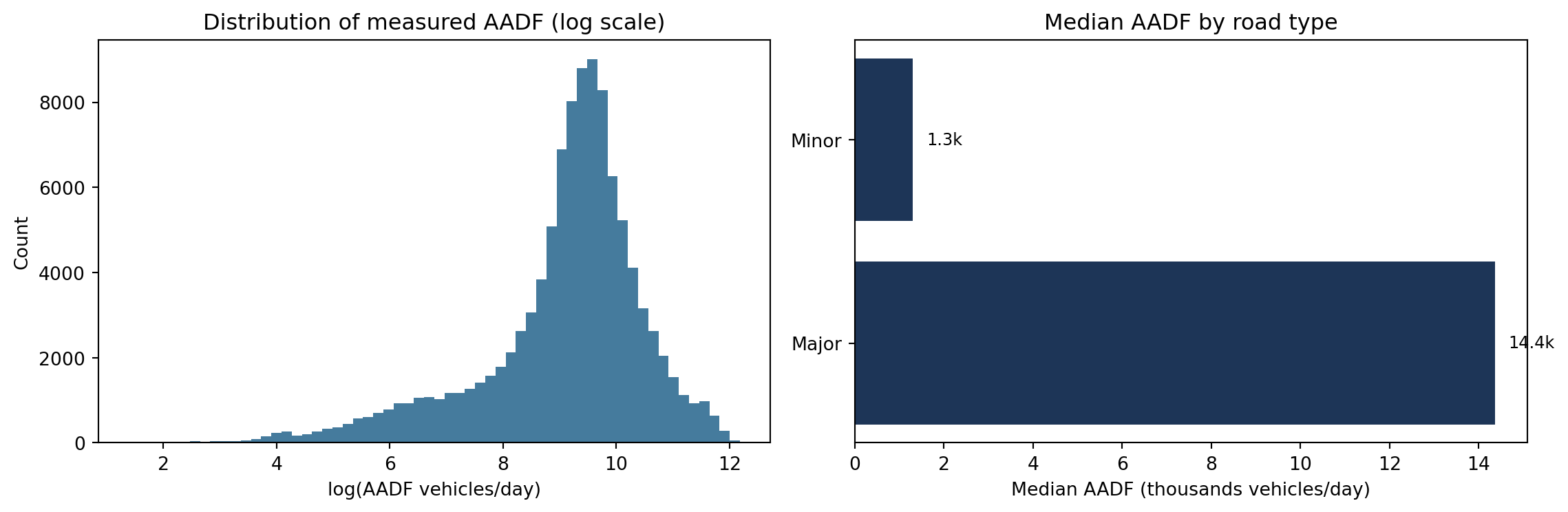
fig, axes = plt.subplots(1, 2, figsize=(12, 4))measured = aadf[aadf["all_motor_vehicles"] >0].copy()axes[0].hist(np.log(measured["all_motor_vehicles"]), bins=60, color="#457b9d", edgecolor="none")axes[0].set_xlabel("log(AADF vehicles/day)")axes[0].set_ylabel("Count")axes[0].set_title("Distribution of measured AADF (log scale)")medians = ( measured.groupby("road_type")["all_motor_vehicles"] .median() .sort_values(ascending=False))axes[1].barh(medians.index, medians.values /1000, color="#1d3557")axes[1].set_xlabel("Median AADF (thousands vehicles/day)")axes[1].set_title("Median AADF by road type")for i, v inenumerate(medians.values): axes[1].text(v /1000+0.3, i, f"{v/1000:.1f}k", va="center", fontsize=9)plt.tight_layout()plt.show()
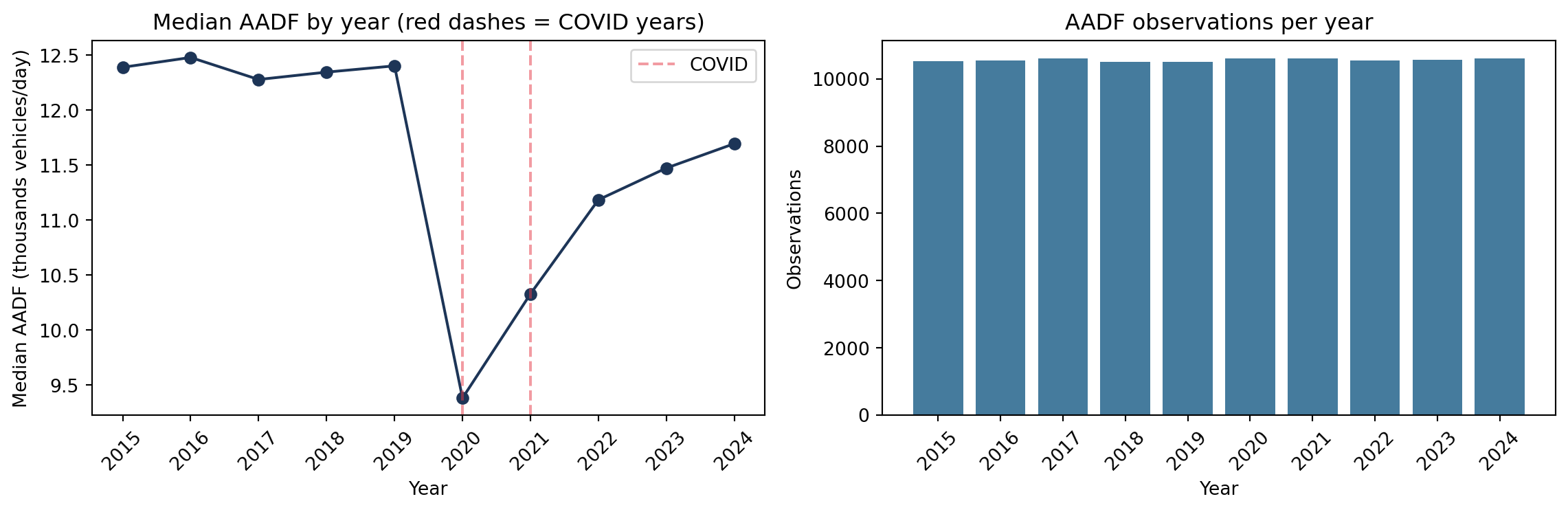
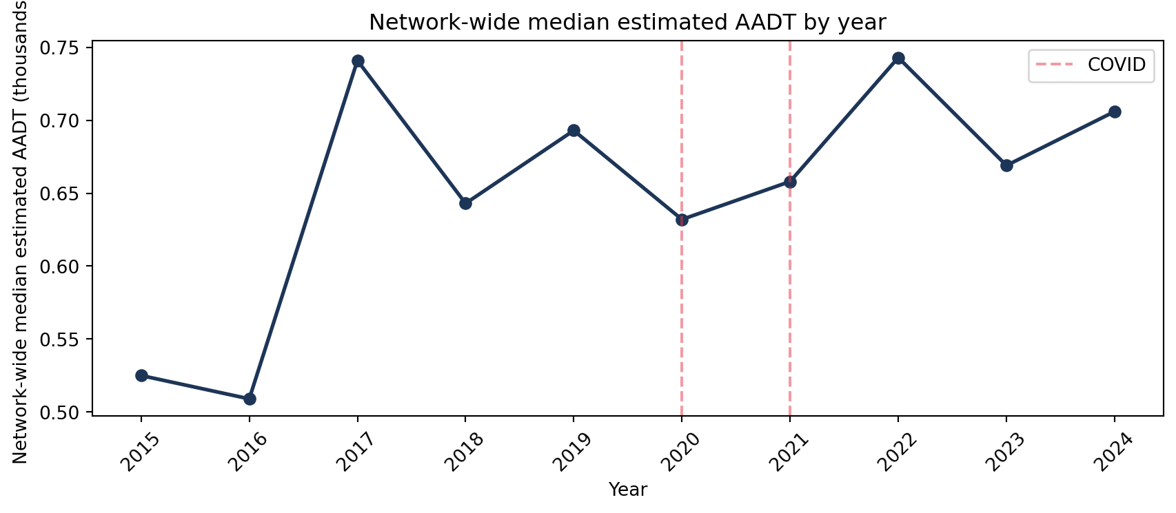
2.3 Annual trends including COVID
year_stats = ( measured.groupby("year")["all_motor_vehicles"] .agg(["median", "count"]) .reset_index())fig, axes = plt.subplots(1, 2, figsize=(12, 4))axes[0].plot(year_stats["year"], year_stats["median"] /1000, marker="o", color="#1d3557")for y in [2020, 2021]:if y in year_stats["year"].values: axes[0].axvline(y, color="#e63946", linestyle="--", alpha=0.5, label="COVID"if y ==2020else"")axes[0].set_xlabel("Year")axes[0].set_ylabel("Median AADF (thousands vehicles/day)")axes[0].set_title("Median AADF by year (red dashes = COVID years)")axes[0].set_xticks(year_stats["year"])axes[0].tick_params(axis="x", rotation=45)axes[0].legend()axes[1].bar(year_stats["year"], year_stats["count"], color="#457b9d")axes[1].set_xlabel("Year")axes[1].set_ylabel("Observations")axes[1].set_title("AADF observations per year")axes[1].set_xticks(year_stats["year"])axes[1].tick_params(axis="x", rotation=45)plt.tight_layout()plt.show()
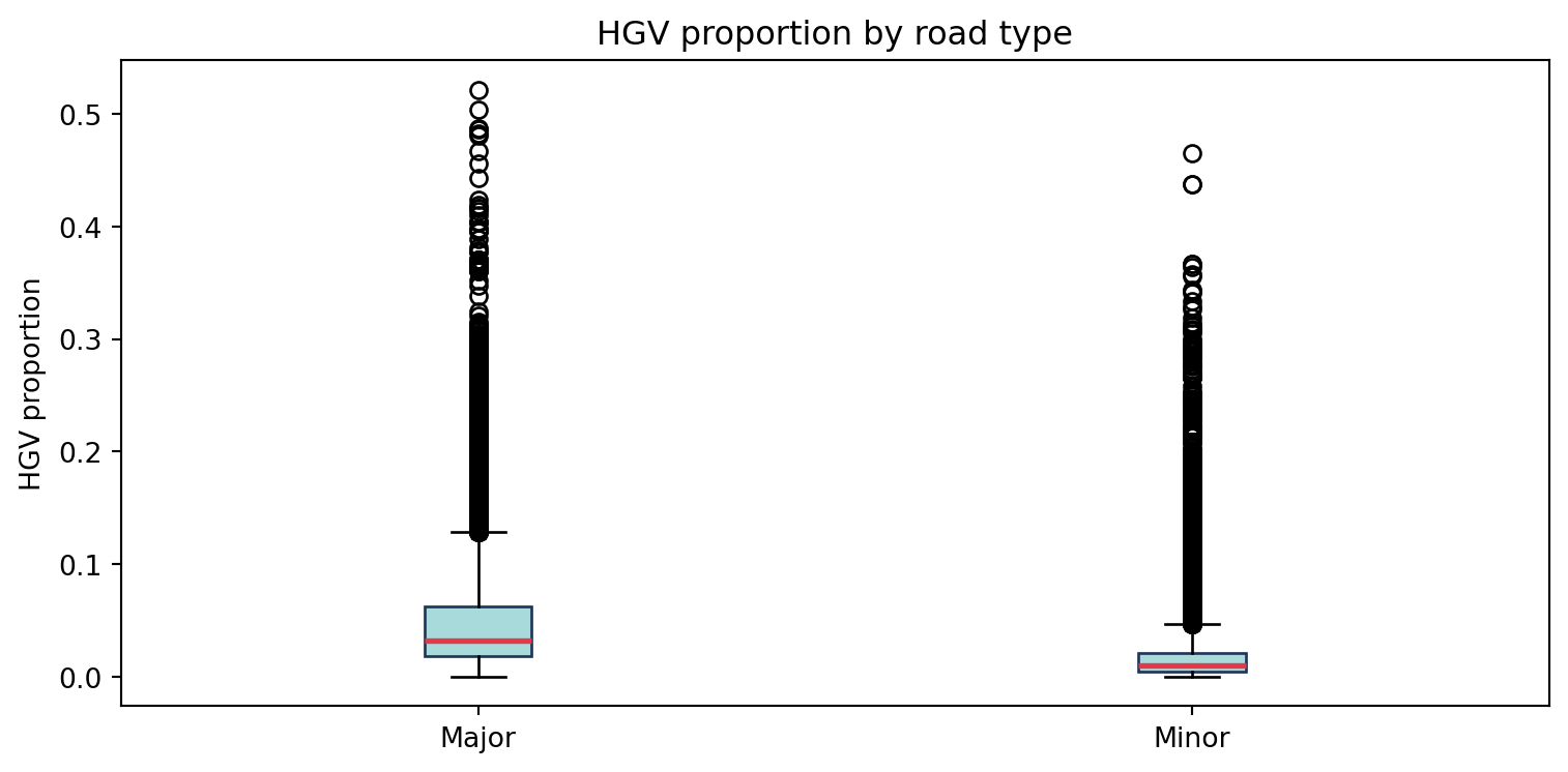
2.4 HGV proportion by road type
hgv_data = measured.dropna(subset=["hgv_proportion", "road_type"])fig, ax = plt.subplots(figsize=(8, 4))road_types = hgv_data["road_type"].value_counts().index.tolist()box_data = [hgv_data[hgv_data["road_type"] == rt]["hgv_proportion"].values for rt in road_types]ax.boxplot(box_data, labels=road_types, patch_artist=True, boxprops=dict(facecolor="#a8dadc", color="#1d3557"), medianprops=dict(color="#e63946", linewidth=2))ax.set_ylabel("HGV proportion")ax.set_title("HGV proportion by road type")plt.tight_layout()plt.show()
3 Stage 1a model
3.1 Design summary
The model is a HistGradientBoostingRegressor (sklearn) with native missing-value handling. The target is log1p(AADF) de-meaned by year so the model learns road-level deviation from the network-wide annual average. Year means are stored separately and added back at inference — this prevents the year feature from dominating importance and collapsing full-network predictions near the annual mean.
GroupKFold CV grouped by count_point_id ensures the same station cannot appear in both train and test folds across years.
WebTRIS flow features are excluded from Stage 1a: they are unavailable for the 2.1M-link network at inference and their absence would need to be imputed with zeros, which corrupts predictions because HistGBR routes NaN and zero through different tree branches.
Feature
Source
road_class_ord
AADF road name prefix (M=6, A=5, B=4, other=1)
is_trunk
road name prefix
latitude, longitude
AADF count point location
is_covid
year flag for 2020–2021
hgv_proportion
AADF vehicle mix
link_length_km
OS Open Roads (snapped via KD-tree)
Network features
betweenness, node degree, dist to major road
3.2 Cross-validation results
metrics_path = ROOT /"data/models/collision_metrics.json"if metrics_path.exists():withopen(metrics_path) as f: all_metrics = json.load(f) aadt_metrics = all_metrics.get("aadt", {})if aadt_metrics:print(f"CV R² : {aadt_metrics['cv_r2_mean']:.3f} (±{aadt_metrics['cv_r2_std']:.3f})")print(f"CV MAE : {aadt_metrics['cv_mae_mean']:.3f} log-units")print(f"n train : {aadt_metrics['n_train']:,}")else:print("No 'aadt' key in collision_metrics.json.")else:print("collision_metrics.json not found — run: python -m road_risk.model --stage traffic")
No 'aadt' key in collision_metrics.json.
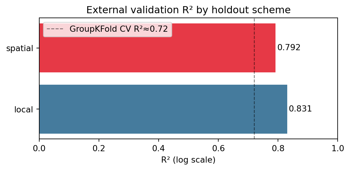
3.3 External validation
Standard CV is optimistic because nearby stations share road class and network context. Two harder holdout schemes probe genuine extrapolation:
Local holdout — 20% of count-point IDs withheld at random. Tests gap-filling.
Spatial block — all points north of the 75th-percentile latitude withheld. Tests generalisation to a region with no measured support.
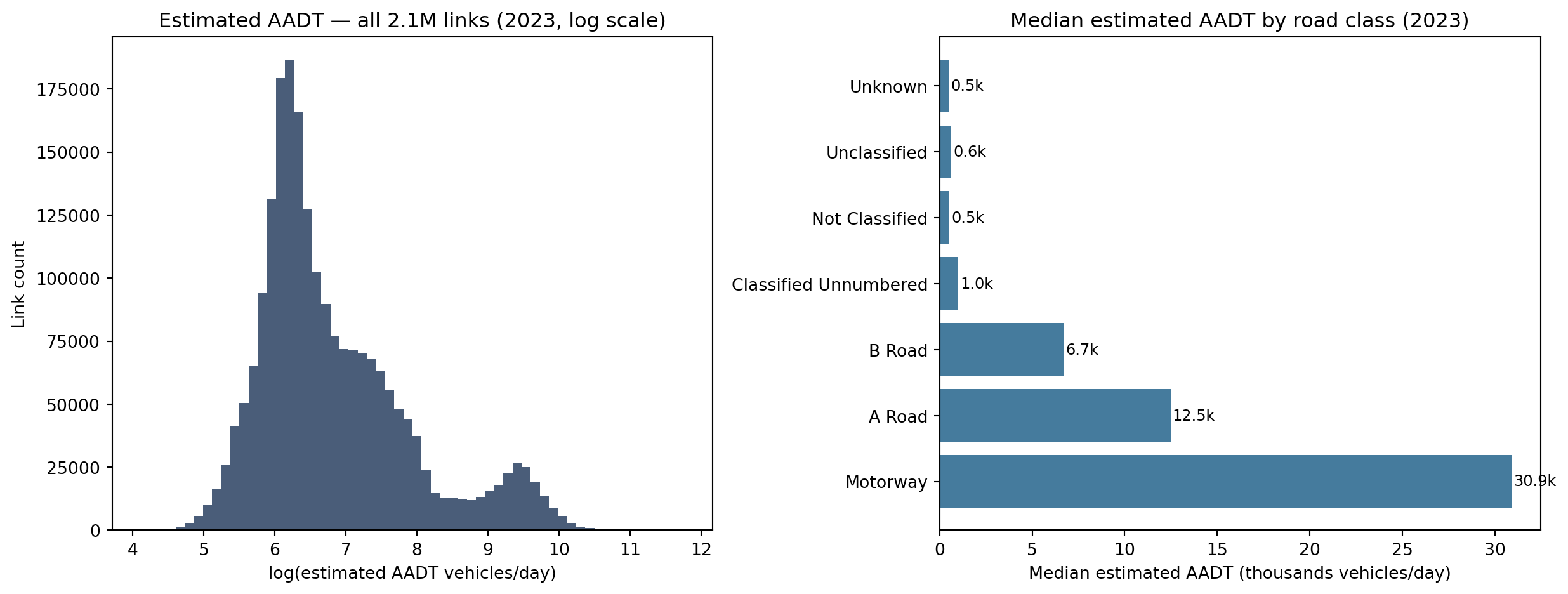
print("=== Stage 1a output summary ===\n")ifnot aadt.empty:print(f"Links with estimates : {aadt['link_id'].nunique():,}")print(f"Years covered : {sorted(aadt['year'].unique())}")print(f"\nEstimated AADT distribution (2023):")print(aadt[aadt['year'] ==2023]['estimated_aadt'].describe().round(0).to_string())ifnot val_summary.empty:print(f"\nExternal validation R²:")for _, row in val_summary.iterrows():print(f" {row['scheme']:10s}: {row['r2']:.3f}")
=== Stage 1a output summary ===

Links with estimates : 2,167,557
Years covered        : [np.int64(2015), np.int64(2016), np.int64(2017), np.int64(2018), np.int64(2019), np.int64(2020), np.int64(2021), np.int64(2022), np.int64(2023), np.int64(2024)]

Estimated AADT distribution (2023):
count    2167557.0
mean        2064.0
std         4129.0
min           60.0
25%          440.0
50%          669.0
75%         1585.0
max       130611.0

External validation R²:
  local     : 0.831
  spatial   : 0.792
Key observations:
The road hierarchy is preserved: motorways and A-roads receive substantially higher AADT than unclassified roads.
COVID years (2020–2021) show a clear network-wide dip consistent with measured AADF.
Local holdout R² exceeds spatial block R², confirming the model is stronger at gap-filling than extrapolating to geography without any measured support.
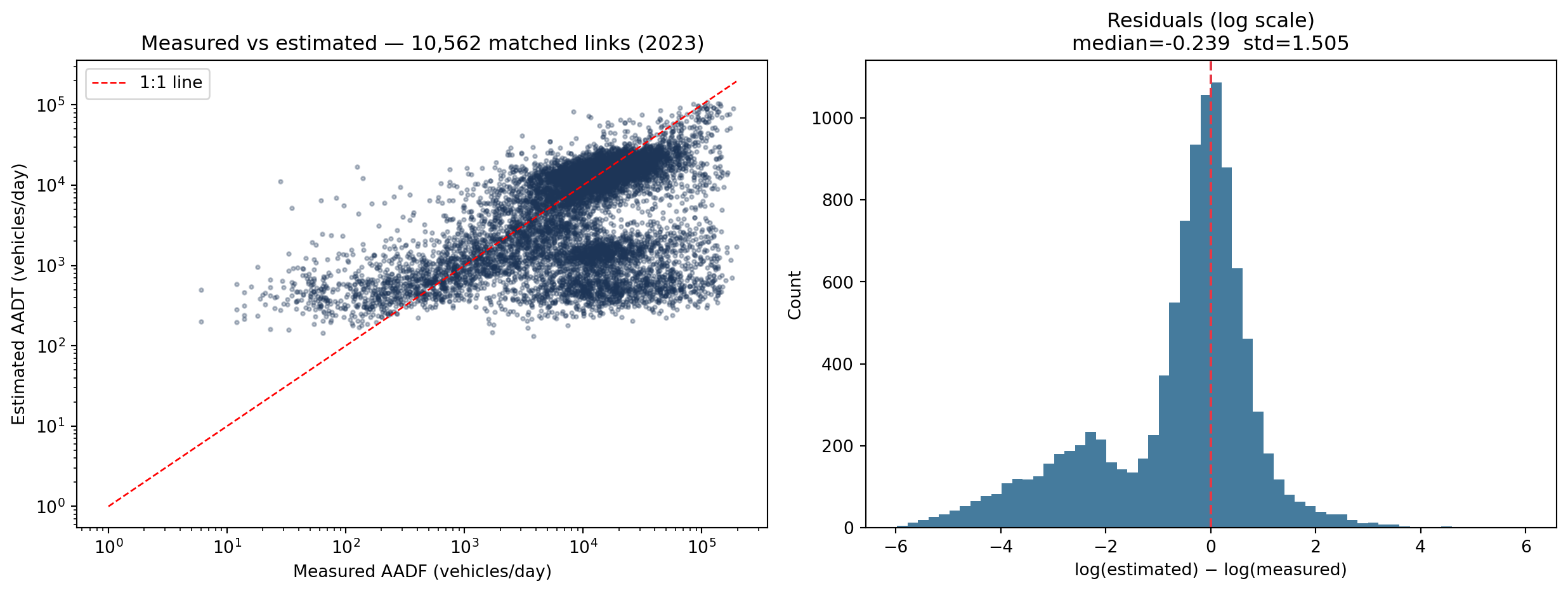
The residual plot for matched links shows approximately zero median bias in log space, with spread driven mainly by minor roads where count-point representativeness is weakest.