Background: Re-evaluating the Collision-Exposure Relationship
A foundational assumption in traditional traffic safety analysis is that risk scales linearly with exposure. Under this assumption, doubling the traffic volume (Annual Average Daily Traffic, or AADT) on a road segment should inherently double the expected number of collisions.
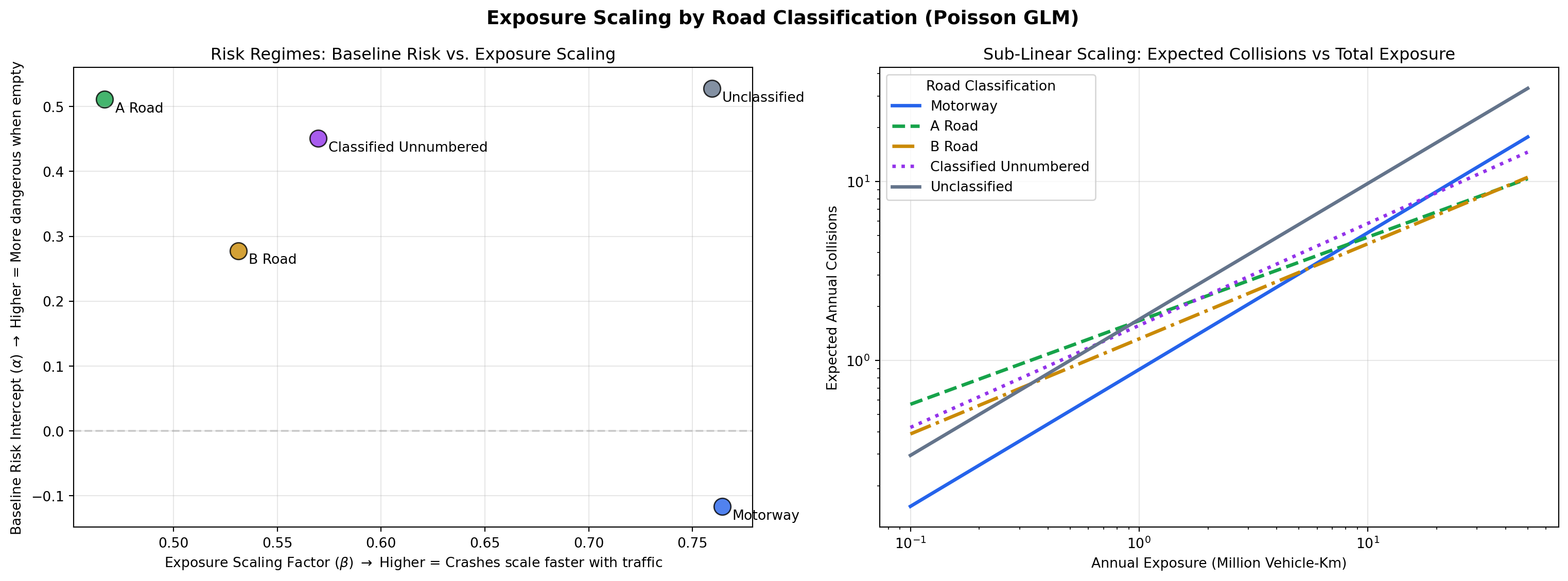
However, when training our count-based network screening model, applying a strict linear exposure offset (base_margin = log_offset) resulted in systematic over-prediction on high-volume roads. To investigate this, we fitted a Poisson Generalized Linear Model (GLM) to the full network—crucially including zero-collision links—to extract the true exposure coefficient (\(\beta\)) for different road characteristics.
The Poisson GLM fits the following relationship:
\[E[Y] = \exp(\alpha + \beta \cdot \ln(\text{Exposure}))\]
Where: * \(E[Y]\) is the expected number of annual collisions. * \(\alpha\) is the baseline risk intercept (how dangerous the road is when nearly empty). * \(\beta\) is the exposure scaling factor. * \(\text{Exposure}\) is the annual vehicle-kilometers travelled on the link.
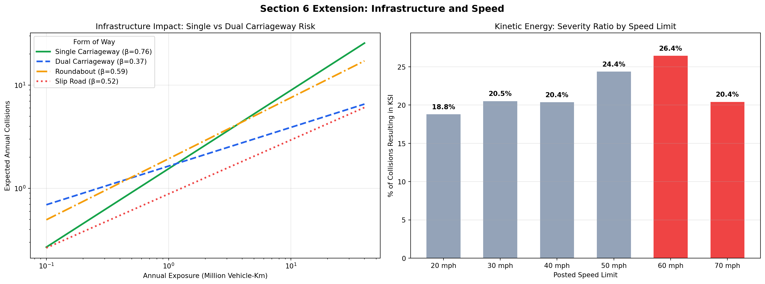
Part 1: Infrastructure Impact (Single vs. Dual Carriageways)
Unclassified: 1060014 links

Classified Unnumbered: 190921 links

Unknown: 442836 links

Not Classified: 224878 links

A Road: 155538 links

B Road: 89286 links

Motorway: 4084 links
| 0 |
Unclassified |
0.677943 |
0.814647 |
| 1 |
Classified Unnumbered |
0.531478 |
0.596444 |
| 2 |
Unknown |
-1.336228 |
0.613607 |
| 3 |
Not Classified |
-1.413974 |
0.633419 |
| 4 |
A Road |
0.505879 |
0.456619 |
| 5 |
B Road |
0.289329 |
0.544913 |
| 6 |
Motorway |
-0.330084 |
0.781436 |
The relationship between traffic volume and collision frequency is not universal; it varies significantly across different road types and forms of way.
- The Single Carriageway Risk Curve (\(\beta = 0.74\)): Single carriageways exhibit a steep exposure scaling curve. While this single-feature GLM confounds infrastructure with other variables (like rural/urban geography and junction density), the descriptive reality remains: adding vehicles to unseparated roads rapidly compounds collision opportunities.
- The Dual Carriageway Flattening Effect (\(\beta = 0.39\)): Dual carriageways show a markedly flatter risk curve. Although they carry a slightly higher baseline risk (α) at very low volumes, the sub-linear scaling demonstrates their capacity to absorb massive increases in traffic volume without a proportional spike in crashes.
Part 2: Kinetic Energy (The 60mph Rural Phenomenon)
While exposure dictates the frequency of collisions, the posted speed limit is a strong proxy for their severity. Mapping the proportion of collisions that result in a Killed or Seriously Injured (KSI) casualty against speed limits reveals a stark descriptive pattern.
- The 60mph Peak (26.4% KSI Rate): The highest severity ratio in the network occurs at 60mph. While speed limit alone confounds other factors (like road class and traffic mix), this matches well-known patterns in UK road safety: 60mph limits are highly prevalent on rural single carriageways, combining high permitted kinetic energy with unseparated opposing flows.
- The 70mph Safety Buffer (20.4% KSI Rate): Despite allowing higher speeds, the severity ratio drops at 70mph. This reflects the reality that 70mph limits are legally restricted almost exclusively to Motorways and high-quality Dual Carriageways, where physical separation mitigates the specific conflict types that make 60mph roads highly severe.
Conclusion: Validating the XGBoost Architecture
These diagnostics reveal a known specification gap in our current v2 architecture. By using log(exposure) as a fixed Poisson offset, the model is effectively forced to assume β=1.
Because the empirical data shows β is actually between 0.4 and 0.8 depending on the road profile, the XGBoost model has to compensate for this misspecification by using other features to artificially absorb the exposure-curvature signal. This likely contributes to the residual variance observed on high-volume networks, and specifically the tendency to under-predict on Motorways.
Recognizing this sub-linear scaling provides a clear diagnostic baseline. It informs our v3 roadmap, where we can empirically test alternative exposure specifications—such as passing log(exposure) as a learned feature, or utilizing per-family fitted GLM offsets—to better capture these realities without forcing the trees to approximate smooth curves.