AADF Traffic Counts

1 Overview

Annual Average Daily Flow (AADF) data provides measured traffic counts at DfT count points across Great Britain. In this project it is the main source of observed exposure: the dataset that anchors traffic estimation before that exposure is extended to roads without direct counts.

This distinction matters. AADF does not provide complete road-link coverage across the network, so it is not the final exposure layer on its own. Instead, it provides the measured foundation for the wider exposure model.

Important

Unlike WebTRIS, which covers the National Highways network only, AADF extends well beyond motorways and trunk roads. That makes it the project’s main source of measured traffic outside the strategic road network, even though coverage is still incomplete.

2 Role in the pipeline

Supplies measured traffic observations that are joined to OS Open Roads links via spatial nearest-neighbour in join.py.
Anchors the exposure story: observed AADF is used where available, and helps justify traffic estimation where direct counts do not exist.
Contributes vehicle-mix features such as HGV proportion and heavy-vehicle share.
Highlights where exposure is directly measured versus modelled — especially on lower-order roads via the estimation_method column.

In short:

AADF is the measured exposure anchor for the project, but not a complete exposure layer for the full network.

3 Download

Source: https://roadtraffic.dft.gov.uk/downloads

The project uses the count point-level AADF dataset, bidirectional aggregate. Place CSVs in data/raw/aadf/.

4 Load data

Code

aadf_path = _ROOT / "data/processed/aadf/aadf_clean.parquet"
aadf = pd.read_parquet(aadf_path)

print(f"rows          : {len(aadf):,}")
print(f"count points  : {aadf['count_point_id'].nunique():,}")
print(f"years         : {sorted(aadf['year'].unique())}")
print(f"road types    : {sorted(aadf['road_type'].dropna().unique())}")

rows          : 105,661
count points  : 14,193
years         : [np.int64(2015), np.int64(2016), np.int64(2017), np.int64(2018), np.int64(2019), np.int64(2020), np.int64(2021), np.int64(2022), np.int64(2023), np.int64(2024)]
road types    : ['Major', 'Minor']

The key thing to keep in mind is that AADF is organised around count points and years, not full road-link coverage. That makes it highly informative where measurements exist, but uneven elsewhere. The page therefore focuses on two questions:

where observed traffic counts exist,
and why those counts are still insufficient on their own for full-network exposure modelling.

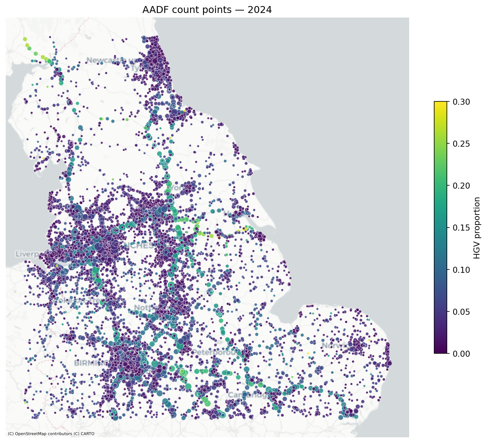
5 Count point coverage

AADF coverage is broader than WebTRIS and extends well beyond the motorway network. Marker size shows traffic volume; colour shows HGV proportion.

This figure is useful less as a map of “all traffic” and more as a map of where the project has measured exposure anchors.

Code

latest = aadf["year"].max()
snap   = aadf[aadf["year"] == latest].copy()
snap   = snap[snap["latitude"].notna() & snap["longitude"].notna()]

gdf = gpd.GeoDataFrame(
    snap,
    geometry=gpd.points_from_xy(snap["longitude"], snap["latitude"]),
    crs="EPSG:4326",
).to_crs(epsg=3857)

minx, miny, maxx, maxy = gdf.total_bounds
pad = max(maxx - minx, maxy - miny) * 0.05

vals = gdf["all_motor_vehicles"]
smin, smax = 8, 120
size_scaled = smin + (smax - smin) * (vals - vals.min()) / (vals.max() - vals.min() + 1e-9)

fig, ax = plt.subplots(figsize=(9, 9))
ax.set_xlim(minx - pad, maxx + pad)
ax.set_ylim(miny - pad, maxy + pad)

try:
    cx.add_basemap(ax, source=cx.providers.CartoDB.Positron,
                   zoom="auto", attribution_size=5)
except Exception as exc:
    print(f"Basemap unavailable: {exc}")

gdf.plot(
    ax=ax, column="hgv_proportion", cmap="viridis",
    markersize=size_scaled, edgecolor="white", linewidth=0.3,
    alpha=0.85, legend=True, zorder=3,
    legend_kwds={"label": "HGV proportion", "shrink": 0.5},
    vmin=0, vmax=max(0.3, gdf["hgv_proportion"].quantile(0.95)),
)
ax.set_axis_off()
ax.set_title(f"AADF count points — {latest}")
plt.tight_layout()
plt.show()

Figure 1: AADF count points — size by flow, colour by HGV share (most recent year)

6 Flow trend over time

AADF flows show the COVID drop clearly — 2020 is ~30% below baseline on most road types, partial recovery in 2021, near-full recovery by 2022.

Code

yearly = (
    aadf.groupby(["year", "road_type"])["all_motor_vehicles"]
    .mean()
    .reset_index()
)

road_types = yearly["road_type"].unique()
colours = plt.cm.tab10(np.linspace(0, 1, len(road_types)))

fig, ax = plt.subplots(figsize=(10, 4.5))
for rt, colour in zip(road_types, colours):
    sub = yearly[yearly["road_type"] == rt]
    ax.plot(sub["year"], sub["all_motor_vehicles"],
            marker="o", linewidth=1.8, label=rt, color=colour)

# Shade COVID years
for yr in COVID_YEARS:
    ax.axvspan(yr - 0.5, yr + 0.5, color="#fee2e2", alpha=0.5, zorder=0)

ax.set_xlabel("Year")
ax.set_ylabel("Mean daily flow (veh/day)")
ax.set_title("AADF mean flow by road type — COVID years shaded")
ax.yaxis.set_major_formatter(mticker.FuncFormatter(lambda x, _: f"{int(x):,}"))
ax.legend(fontsize=8, loc="best")
ax.spines[["top", "right"]].set_visible(False)
ax.grid(alpha=0.2)
plt.tight_layout()
plt.show()

Figure 2: Mean daily flow by road type over time

7 Flow and vehicle mix by road type

Summary at the most recent year. estimation_method indicates whether flow was directly counted or modelled — minor roads are mostly modelled.

Code

summary = (
    snap.groupby("road_type")
    .agg(
        n_count_points       =("count_point_id",    "nunique"),
        mean_daily_flow      =("all_motor_vehicles", "mean"),
        mean_hgv_flow        =("all_hgvs",           "mean"),
        mean_hgv_share_pct   =("hgv_proportion",     lambda x: 100 * x.mean()),
        mean_heavy_share_pct =("heavy_vehicle_prop", lambda x: 100 * x.mean()),
    )
    .round(1)
    .sort_values("mean_daily_flow", ascending=False)
)
display(summary)

	n_count_points	mean_daily_flow	mean_hgv_flow	mean_hgv_share_pct	mean_heavy_share_pct
road_type
Major	8293	22166.7	1381.2	4.4	19.5
Minor	2322	2865.8	33.7	1.8	16.2

Code

if "estimation_method" in aadf.columns:
    est = (
        snap.groupby(["road_type", "estimation_method"])
        .size()
        .unstack(fill_value=0)
    )
    display(est)

estimation_method	Counted	Estimated
road_type
Major	1936	6357
Minor	1874	448

8 Variables and model use

AADF column	Description	Used in model
`all_motor_vehicles`	Total motor vehicle daily flow	`log_motor_vehicles`, rate denominator
`all_hgvs`	HGV daily flow	`log_hgv_daily`
`hgv_proportion`	HGV share (0–1)	`hgv_pct_aadf`
`heavy_vehicle_prop`	All heavy vehicles (HGV + bus) share	feature
`link_length_km`	Road link length	rate denominator (veh-km)
`road_type`	Motorway / A / B / minor	ordinal encoding + flags
`estimation_method`	Counted vs modelled	confidence flag (not currently used)

The rate calculation in features.py is:

collision_rate_per_mvkm = collisions / (all_motor_vehicles × link_length_km × 365 / 1e6)

9 Why this source is not enough on its own

AADF is the strongest directly observed traffic dataset in the pipeline, but it is still incomplete in three important ways:

it is count-point based rather than full road-link coverage,
it is stronger on major roads than local roads,
and only a subset of years may be active in the current modelling workflow.

That is why the project does not stop at joining AADF onto road links. Instead, AADF is used to support the traffic exposure model, which estimates AADT beyond the measured network. ***

10 Known issues and limitations

Bidirectional aggregate — the clean AADF has flows summed across both directions. Directional analysis would require re-running the raw ingest.
Modelled vs counted flow — many minor-road AADFs are modelled from nearby counts. The estimation_method column indicates which. Modelled values are less reliable, particularly for HGV proportion.
Count point drift — count point locations occasionally move between years. The project uses nearest-neighbour spatial join rather than point ID matching to handle this, at the cost of some precision.
Temporal granularity — annual aggregates only. WebTRIS is required for any sub-annual analysis and covers only major roads.
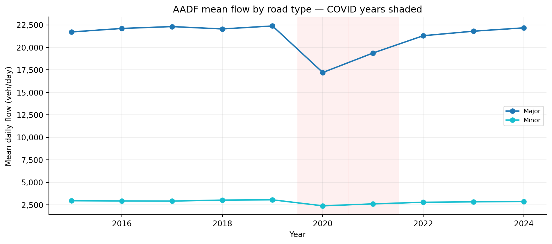
COVID — 2020 flows are substantially suppressed. is_covid flag carried through the pipeline allows exclusion or separate modelling of these years.

11 Next steps

AADF feeds into:

join.py → spatial nearest-neighbour onto OS Open Roads links (2km cap)
features.py → traffic volume and vehicle mix features
collision rate denominator via link_length_km × all_motor_vehicles × 365