Source notes for WebTRIS sensor data used to study traffic timing, vehicle mix, and time-zone profiles on major roads.
1 Why this matters
Important
WebTRIS provides measured traffic data on major roads. In this project it is used to add real observations — particularly vehicle mix and corridor behaviour — to a pipeline that otherwise relies on partial counts and modelling.
Most datasets in transport either describe the network (roads, geometry) or outcomes (collisions). WebTRIS is different: it measures what is actually happening on the road — but only at specific sensor locations.
2 What this page answers
What is WebTRIS and how is it used in practice?
How is the data physically measured?
Where are the sites and what years are covered?
How do flows vary seasonally and by weekday?
How concentrated is traffic within the working day?
What do these variables mean for the model?
3 Use in practice
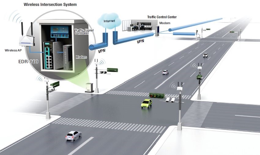
WebTRIS is a traffic sensor system used by National Highways to monitor and manage conditions on the Strategic Road Network, including congestion and incident response.1
It is used in planning and analytical work — Department for Transport studies use it to analyse how traffic changes over time, for example in work on induced demand.2 In safety and evaluation studies it is combined with collision data (e.g. STATS19) to assess how risk varies across the network.3 In modelling contexts it is used to calibrate traffic models and estimate heavy vehicle flows for infrastructure analysis.45
A common use is to define typical traffic conditions, where sensor data is filtered to remove anomalies and aggregated to represent baseline behaviour.6
WebTRIS is not used to represent the whole network. It provides measured reference points on major roads that support analysis and modelling.
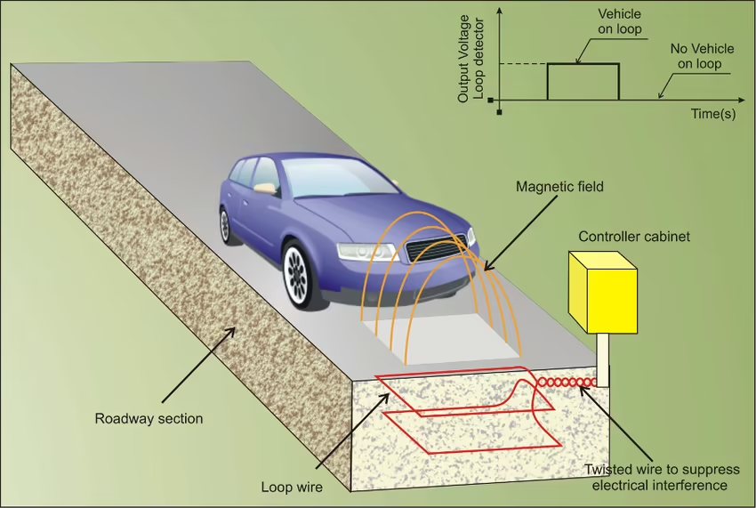
WebTRIS data is primarily collected using inductive loop detectors embedded in the road surface. These sensors detect vehicles by measuring changes in an electromagnetic field as metal passes over the loop. From this, the system derives vehicle counts, speed (from multiple loops), and vehicle length (estimated from time over the sensor).
Vehicle type is not directly observed — it is inferred from length bands.
sites = pd.read_parquet(sites_path) if sites_path.exists() else pd.DataFrame()webtris = pd.read_parquet(webtris_path) if (webtris_path isnotNoneand webtris_path.exists()) else pd.DataFrame()time_webtris = pd.read_parquet(time_webtris_path) if time_webtris_path.exists() else pd.DataFrame()# Normalise year column — ingest output uses _pull_year; clean output uses yearifnot webtris.empty and"_pull_year"in webtris.columns and"year"notin webtris.columns: webtris = webtris.rename(columns={"_pull_year": "year"})# Resolve column name variants between ingest and clean outputsCOL_FLOW =next((c for c in ["adt24hour", "mean_daily_flow", "all_flow"] if c in webtris.columns), None)COL_WD_FLOW =next((c for c in ["awt24hour", "mean_weekday_flow", "weekday_flow"] if c in webtris.columns), None)COL_LV =next((c for c in ["adt24largevehiclepercentage", "large_vehicle_pct", "hgv_pct"] if c in webtris.columns), None)COL_LV_WD =next((c for c in ["awt24largevehiclepercentage", "large_vehicle_weekday_pct", "hgv_weekday_pct"] if c in webtris.columns), None)# WebTRIS API often returns object dtype — convert once hereifnot webtris.empty: webtris["year"] = pd.to_numeric(webtris["year"], errors="coerce").astype("Int64")if"monthname"in webtris.columns: webtris["monthname"] = webtris["monthname"].map(normalise_month)for col in [COL_FLOW, COL_WD_FLOW, COL_LV, COL_LV_WD]:if col: webtris[col] = pd.to_numeric(webtris[col], errors="coerce")webtris["year"] = webtris["year"].astype(int)YEAR_COLOURS = make_year_colours(webtris["year"].dropna().unique())print(f"sites rows : {len(sites):,}")print(f"webtris rows : {len(webtris):,}")print(f"\nResolved columns:")print(f" flow (all-day) : {COL_FLOW}")print(f" flow (weekday) : {COL_WD_FLOW}")print(f" large veh % : {COL_LV}")print(f" large veh % WD : {COL_LV_WD}")if"monthname"in webtris.columns:print(f" months present : {sorted(webtris['monthname'].dropna().unique().tolist())}")print(f" years present : {sorted(webtris['year'].dropna().unique().tolist())}")
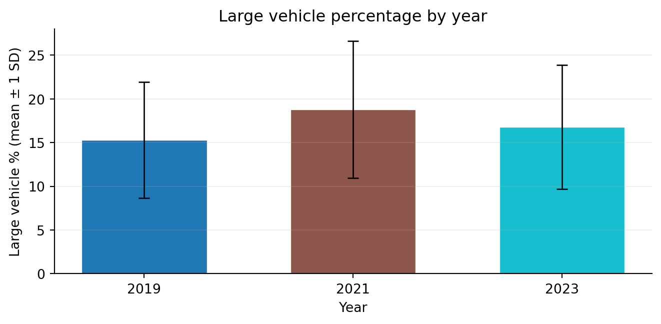
Figure 2: Mean large vehicle percentage by year (± 1 SD across sites)
 year      mean      std    n
 2019 15.304335 6.615736 4766
 2021 18.784249 7.851997 5097
 2023 16.766444 7.091977 5148
Large vehicle percentage is broadly stable across years — the motorway network composition does not change quickly. Error bars reflect variation across sites (some corridors are much more freight-heavy than others) rather than measurement uncertainty.
8 Seasonal flow patterns
Monthly flow data is available in the annual reports file. The grey line shows mean all-day flow by month; the red dashed line (right axis) shows how much higher weekday flows are relative to the all-day average for that month.
Code
if"monthname"notin webtris.columns:print("'monthname' not present — data is likely at annual grain, not monthly.")else: months_present = [m for m in MONTH_ORDER if m in webtris["monthname"].unique()] xticks =range(len(months_present)) xlabels = months_present month_avg = ( webtris.groupby("monthname", observed=True) .agg({COL_FLOW: "mean", COL_WD_FLOW: "mean", COL_LV: "mean", COL_LV_WD: "mean"}) .reindex(months_present) .reset_index() .rename(columns={ COL_FLOW: "mean_flow", COL_WD_FLOW: "mean_weekday_flow", COL_LV: "large_vehicle_pct", COL_LV_WD: "large_vehicle_weekday_pct", }) ) flow_delta = ( (month_avg["mean_weekday_flow"] - month_avg["mean_flow"])/ month_avg["mean_flow"] *100 ) lv_delta = ( (month_avg["large_vehicle_weekday_pct"] - month_avg["large_vehicle_pct"])/ month_avg["large_vehicle_pct"] *100 ) fig, axes = plt.subplots(1, 2, figsize=(12, 4)) ax0, ax0R = axes[0], axes[0].twinx() ax0.plot(xticks, month_avg["mean_flow"], color=AVERAGE_COLOUR, marker="o", linewidth=1.8, label="All-day avg") ax0R.plot(xticks, flow_delta, color=DELTA_COLOUR, marker="o", linewidth=1.5, linestyle="--", label="Weekday premium") ax0.set_xticks(xticks) ax0.set_xticklabels(xlabels, rotation=45, ha="right", fontsize=8) ax0.set_ylabel("Mean daily flow (veh/day)") ax0R.set_ylabel("Weekday vs all-day premium (%)") ax0.set_ylim(0, month_avg["mean_flow"].max() *1.2) ax0R.set_ylim(0, flow_delta.max() *1.5) ax0.set_title("Total flow") ax0.spines[["top"]].set_visible(False) ax0.grid(alpha=0.2) lines = ax0.get_lines() + ax0R.get_lines() ax0.legend(lines, [l.get_label() for l in lines], fontsize=8) ax1, ax1R = axes[1], axes[1].twinx() ax1.plot(xticks, month_avg["large_vehicle_pct"], color=AVERAGE_COLOUR, marker="o", linewidth=1.8, label="All-day LV%") ax1R.plot(xticks, lv_delta, color=DELTA_COLOUR, marker="P", linewidth=1.5, linestyle="--", label="Weekday premium") ax1.set_xticks(xticks) ax1.set_xticklabels(xlabels, rotation=45, ha="right", fontsize=8) ax1.set_ylabel("Large vehicle %") ax1R.set_ylabel("Weekday LV vs all-day premium (%)") ax1.set_ylim(0, month_avg["large_vehicle_pct"].max() *1.2) ax1R.set_ylim(0, lv_delta.max() *1.5) ax1.set_title("Large vehicle %") ax1.spines[["top"]].set_visible(False) ax1.grid(alpha=0.2) lines = ax1.get_lines() + ax1R.get_lines() ax1.legend(lines, [l.get_label() for l in lines], fontsize=8) fig.suptitle("Seasonal patterns — network average across all years", y=1.02) plt.tight_layout() plt.show()
'monthname' not present — data is likely at annual grain, not monthly.
Figure 3
Reading the chart: The grey line (left axis) shows the seasonal shape of traffic volume — typically a summer peak, January trough. The red dashed line (right axis) is the weekday premium: how many percent more traffic flows on weekdays compared to the 7-day all-day average for that month. The right panel repeats this for large vehicle percentage — a consistently positive weekday premium means HGV flows are concentrated on working days regardless of season.
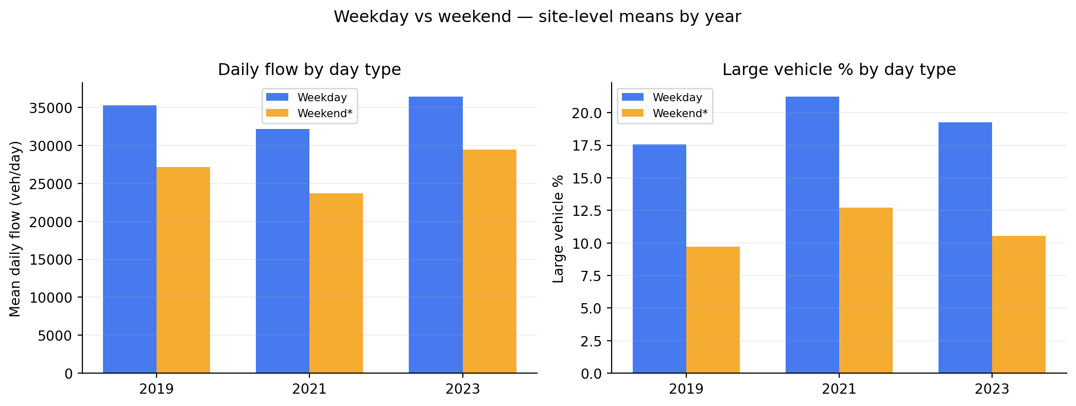
9 Weekday vs weekend
Weekday daily average is directly available. Weekend flow is estimated as the complement: (7 × all-day − 5 × weekday) / 2.
Code
webtris["est_weekend_flow"] = (7* webtris[COL_FLOW] -5* webtris[COL_WD_FLOW]) /2webtris["est_weekend_lv"] = (7* webtris[COL_LV] -5* webtris[COL_LV_WD]) /2years =sorted(webtris["year"].dropna().unique())x = np.arange(len(years))width =0.35fig, axes = plt.subplots(1, 2, figsize=(11, 4))wd_means = [webtris.loc[webtris["year"] == yr, COL_WD_FLOW].mean() for yr in years]we_means = [webtris.loc[webtris["year"] == yr, "est_weekend_flow"].mean() for yr in years]axes[0].bar(x - width/2, wd_means, width, label="Weekday", color="#2563eb", alpha=0.85)axes[0].bar(x + width/2, we_means, width, label="Weekend*", color="#f59e0b", alpha=0.85)axes[0].set_xticks(x)axes[0].set_xticklabels([str(yr) for yr in years])axes[0].set_ylabel("Mean daily flow (veh/day)")axes[0].set_title("Daily flow by day type")axes[0].legend(fontsize=8)axes[0].spines[["top", "right"]].set_visible(False)axes[0].grid(axis="y", alpha=0.2)wd_lv = [webtris.loc[webtris["year"] == yr, COL_LV_WD].mean() for yr in years]we_lv = [webtris.loc[webtris["year"] == yr, "est_weekend_lv"].mean() for yr in years]axes[1].bar(x - width/2, wd_lv, width, label="Weekday", color="#2563eb", alpha=0.85)axes[1].bar(x + width/2, we_lv, width, label="Weekend*", color="#f59e0b", alpha=0.85)axes[1].set_xticks(x)axes[1].set_xticklabels([str(yr) for yr in years])axes[1].set_ylabel("Large vehicle %")axes[1].set_title("Large vehicle % by day type")axes[1].legend(fontsize=8)axes[1].spines[["top", "right"]].set_visible(False)axes[1].grid(axis="y", alpha=0.2)fig.suptitle("Weekday vs weekend — site-level means by year", y=1.02)plt.tight_layout()plt.show()print("* Weekend estimated as (7 × all-day − 5 × weekday) / 2")
Figure 4: Weekday vs estimated weekend flow and large vehicle % by year
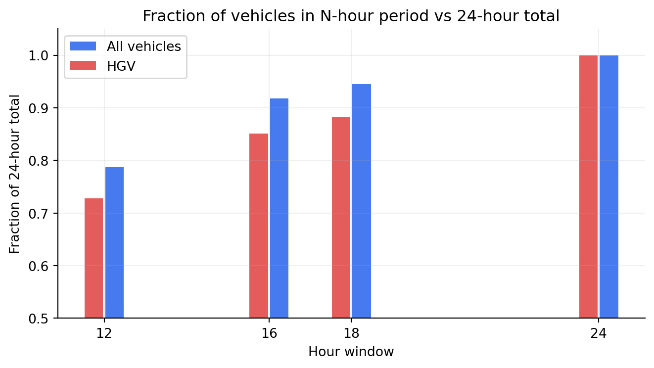
The time_webtris dataset contains sub-24h flow averages for 12, 16, and 18-hour windows. These give a rough picture of how concentrated flows are within the working day — useful for understanding what the annual average masks.
Code
frac_means = time_webtris[frac_cols].mean()adt_hgv, adt_all = [], []for col in frac_cols: hours =int(col.split("hour")[0].split("t")[-1]) val = frac_means[col]if"adt"notin col:continue (adt_hgv if col.endswith("_hgv") else adt_all).append((hours, val))adt_hgv = np.array(sorted(adt_hgv))adt_all = np.array(sorted(adt_all))fig, ax = plt.subplots(figsize=(7, 4))ax.bar(adt_all[:, 0] +0.25, adt_all[:, 1], width=0.45, label="All vehicles", color="#2563eb", alpha=0.85)ax.bar(adt_hgv[:, 0] -0.25, adt_hgv[:, 1], width=0.45, label="HGV", color="#dc2626", alpha=0.75)ax.set_xlabel("Hour window")ax.set_ylabel("Fraction of 24-hour total")ax.set_title("Fraction of vehicles in N-hour period vs 24-hour total")ax.set_xticks([12, 16, 18, 24])ax.set_ylim(0.5, 1.05)ax.legend()ax.grid(alpha=0.2)ax.spines[["top", "right"]].set_visible(False)plt.tight_layout()plt.show()
Figure 5: Fraction of 24-hour traffic captured in N-hour windows
Code
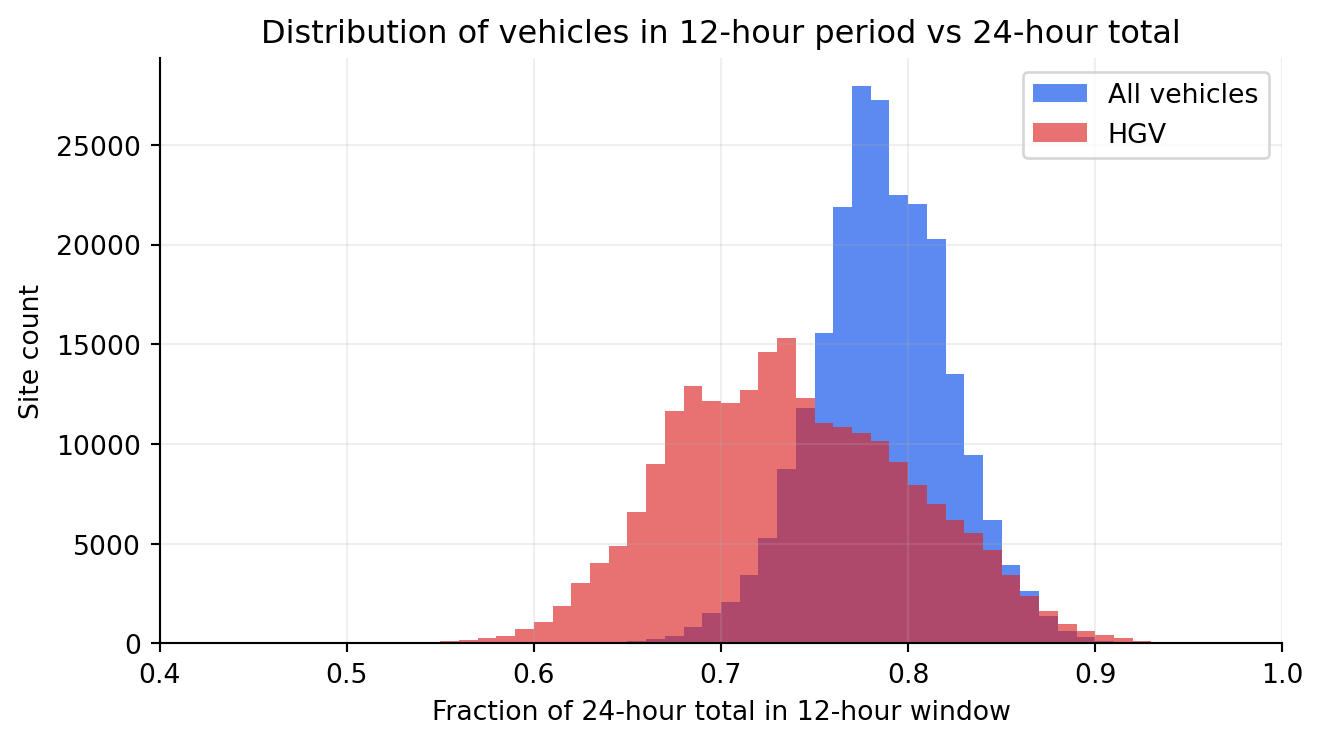
fig, ax = plt.subplots(figsize=(7, 4))bins = np.arange(0.4, 1.01, 0.01)time_webtris["frac_awt12hour"].hist( bins=bins, ax=ax, label="All vehicles", color="#2563eb", alpha=0.75)time_webtris["frac_awt12hour_hgv"].hist(bins=bins, ax=ax, label="HGV", color="#dc2626", alpha=0.65)ax.set_xlabel("Fraction of 24-hour total in 12-hour window")ax.set_ylabel("Site count")ax.set_title("Distribution of vehicles in 12-hour period vs 24-hour total")ax.set_xlim(0.4, 1.0)ax.legend()ax.grid(alpha=0.2)ax.spines[["top", "right"]].set_visible(False)plt.tight_layout()plt.show()
Figure 6: Distribution of 12-hour fraction across sites (all vehicles vs HGV)
Most sites see roughly 70–80% of daily traffic in the 12-hour core window. The HGV distribution shifted right relative to all vehicles means heavy goods vehicles are more concentrated in daytime hours — consistent with delivery restrictions and driver hours regulations.
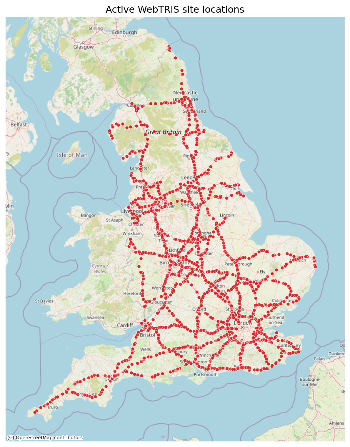
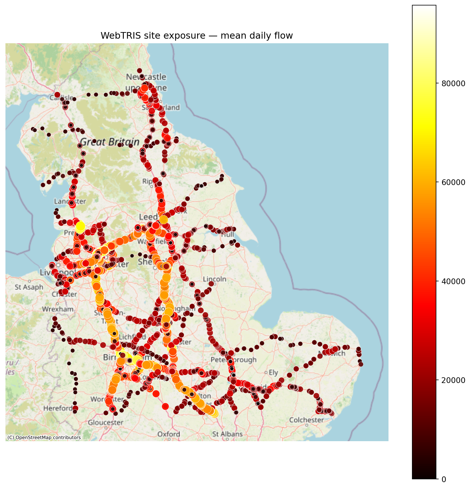
11 Site exposure maps
Flow and large vehicle percentage vary across the network. The maps below show site-level means, sized and coloured by the chosen variable.
Code
active = prepare_webtris_site_exposure( sites, webtris, exposure_columns=[COL_FLOW, COL_WD_FLOW])plot_webtris_site_exposure( active, value_col=COL_FLOW, cmap="hot", title="WebTRIS site exposure — mean daily flow", colorbar_label="Mean daily flow (veh/day)",)
Figure 7: Mean all-day daily flow by site
Code
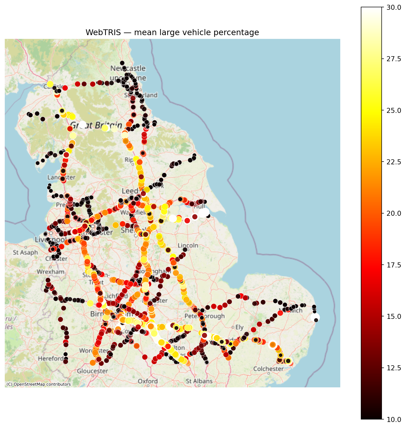
active = prepare_webtris_site_exposure( sites, webtris, exposure_columns=[COL_LV, COL_LV_WD])plot_webtris_site_exposure( active, value_col=COL_LV, cmap="hot", clim=(10, 30), title="WebTRIS — mean large vehicle percentage", colorbar_label="Large vehicle %",)
Figure 8: Mean large vehicle percentage by site
12 Variables and model use
WebTRIS annual report columns follow the pattern [a][d/w]t[hours][metric]: a = average, d = all days, w = weekday, t = traffic, hours = window length.
Raw report field
Clean field
Meaning
adt24hour
all_flow
Mean daily flow, all days, 24h
awt24hour
weekday_flow
Mean daily flow, weekdays, 24h
adt24largevehiclepercentage
hgv_pct
Large vehicle share, all days
awt24largevehiclepercentage
hgv_weekday_pct
Large vehicle share, weekdays
adt12hour, adt16hour, etc.
all_flow_12h, all_flow_16h, etc.
Flow in N-hour window
NoteWhat better features could look like
The current profile model uses annual and N-hour aggregates rather than raw 15-minute sensor traces. Richer features would require additional data pulls:
Time-of-day — pull_site_year_daily() in ingest_webtris.py fetches 15-minute interval data. Peak-hour flow, AM/PM ratios, and night-time HGV share could all be derived from it. Each site-year requires ~176 API requests so this is practical only for a targeted sample of sites.
Weekday-stratified HGV risk — hgv_weekday_pct is already in the cleaned table but not used as a separate Stage 2 feature. If risk is being modelled for weekday conditions specifically, this is a better input than the all-day figure.
Peak/off-peak ratio — the 12h/16h/18h windows in time_webtris approximate the core operating day. A peak/off-peak ratio would separate commuter corridors from 24-hour freight routes, which likely have different risk profiles.
WebTRIS covers the National Highways network only — motorways and major trunk roads. The webtris_available flag in features.py is True for a small minority of road links. Any feature using WebTRIS columns will have high missingness across the wider network. This is a structural property of the data source, not a processing error.
14 Key assumptions and limitations
Motorway sensors are taken to represent their corridor — there is no spatial interpolation to nearby roads.
Vehicle type is inferred from loop-detected length, not directly observed.
Annual averages mask intra-day variation. The 12h/16h fractions suggest roughly 70–80% of flow occurs in the core working day.
Sparse year sampling means trends between sampled years are not directly observable.
The sparse pull uses 2019, 2021, and 2023. This captures one COVID-period year but not the full 2020 shock or year-by-year recovery.